Two-Way ANCOVA (RBD)
Description: This tutorial provides a comprehensive guide to understanding and conducting a two-way Analysis of Covariance (ANCOVA) within a Randomized Block Design (RBD). We detail the mathematical formulation, underlying statistical assumptions, and practical steps for interpreting estimated marginal means and model diagnostics in RAISINS. Read more …
Analysis of Covariance (ANCOVA) blends analysis of variance with regression: it compares treatment means the way ANOVA does, but first removes the influence of a continuous variable, the covariate, that would otherwise effect the comparison. ANCOVA (RBD), accounts for two sources of variance at once, the treatments under study and the blocks (replications) they are grouped in, while adjusting every treatment mean for the covariate. This tutorial introduces the conceptual parts very briefly and It then walks through the complete analysis in RAISINS, including the ANCOVA table, covariate-adjusted (estimated marginal) means with letter groupings, pairwise comparisons, a PCA-based multivariate index, residual normality checks, publication-ready plots, and AI-assisted interpretation, all without writing a single line of code.
1 Introduction and Theoretical Motivation
In agricultural field experiments, researchers often compare the average performance of different treatments, such as the yield of crop varieties. However, these comparisons can sometimes be misleading because the experimental plots may differ naturally in factors such as soil fertility, moisture, or the initial size and vigour of plants. These differences can affect the results even if the treatments themselves are equally effective.
For example, suppose a trial compares 5 mango varieties across 4 replications. The average yield of Alphonso is about 1427 kg, while Safeda averages about 1060 kg. At first glance, Alphonso appears to be the better variety. However, if the Alphonso trees were already larger or growing in more fertile plots before the experiment, part of its higher yield may be due to these favourable conditions rather than the variety itself. Therefore, comparing simple averages alone may not provide a fair comparison of the treatments.
A covariate (\(x\)) is a continuous variable measured before or after the application of treatments that is not affected by the treatments but exhibits a linear relationship with the response variable under study. Failure to account for a relevant covariate may result in two distinct analytical errors:
- Bias. A mediocre treatment that enjoyed a superior baseline appears artificially effective, while a good treatment on poor plots is unfairly penalised.
- Inflated error variance. Variation the covariate could have explained is left inside the residual error term, reducing statistical power and masking genuine treatment effects.
An Analysis of Covariance (ANCOVA) resolves both by combining analysis of variance with linear regression. It evaluates treatment effects after mathematically adjusting every observation to what it would have been at a common covariate value, namely the grand covariate mean \(\bar{x}\). The adjusted estimates it produces are the Estimated Marginal Means (EMMs), the honest, like-for-like counterparts of the raw averages, and they are the values RAISINS reports, letters, and plots. The term “two-way” refers to the two structural factors the model recognises before any covariate adjustment: the treatments under study and the blocks (replications) of the Randomized Block Design (RBD).
| Method | What it compares | Role of the covariate |
|---|---|---|
| ANOVA | Treatment means only | Ignored entirely |
| Regression | The response against a continuous predictor | Is the predictor; no treatment groups |
| ANCOVA | Treatment means, adjusted for a continuous predictor | Included as a nuisance variable to be removed |
A two-way ANCOVA compares treatment means in a blocked field trial after statistically equating every plot on a continuous covariate, so the comparison reflects the treatments themselves rather than the conditions in which they happened to grow.
A covariate should be (1) continuous, (2) measured before the treatments could affect it, or otherwise genuinely independent of them, and (3) related to the response. Initial plant height, pre-treatment soil nutrient level, tree girth, or a baseline count are classic examples. A variable that is itself changed by the treatment is a poor covariate: adjusting for it would remove part of the very treatment effect you are trying to measure.
2 Mathematical Framework and Model Specification
In a two-way layout with a Randomized Block Design, the total variation in the response is partitioned into two structural components (treatments and blocks), one continuous linear component (the covariate), and residual error. The formal model makes each of these explicit.
2.1 The statistical model
The linear model for a two-way ANCOVA in an RBD with a single continuous covariate is
\[y_{ij} = \mu + \tau_i + \beta_j + \gamma\,(x_{ij} - \bar{x}) + \varepsilon_{ij}\]
where
- \(y_{ij}\) is the observed response for treatment \(i\) \((i = 1, 2, \dots, t)\) in block \(j\) \((j = 1, 2, \dots, b)\);
- \(\mu\) is the overall population mean response;
- \(\tau_i\) is the effect of the \(i\)-th treatment, subject to \(\sum_i \tau_i = 0\);
- \(\beta_j\) is the effect of the \(j\)-th block, subject to \(\sum_j \beta_j = 0\);
- \(\gamma\) is the common regression coefficient (slope) relating the covariate to the response;
- \(x_{ij}\) is the covariate value for treatment \(i\) in block \(j\), and \(\bar{x}\) is its grand mean;
- \(\varepsilon_{ij}\) is the random error, assumed \(\varepsilon_{ij} \sim \text{NID}(0, \sigma^2)\).
The term \(\gamma\,(x_{ij} - \bar{x})\) is the covariate adjustment; it is precisely what distinguishes ANCOVA from a plain two-way ANOVA.
2.2 Covariate adjustment and estimated marginal means
Once the pooled slope \(\hat{\gamma}\) has been estimated from the data, the adjusted (estimated marginal) mean for the \(i\)-th treatment is
\[\hat{\mu}_i^{\text{adj}} = \bar{y}_{i\cdot} - \hat{\gamma}\,(\bar{x}_{i\cdot} - \bar{x})\]
where \(\bar{y}_{i\cdot}\) and \(\bar{x}_{i\cdot}\) are the unadjusted sample means of the response and the covariate for treatment \(i\). In words, a treatment whose plots enjoyed an above-average covariate value (\(\bar{x}_{i\cdot} > \bar{x}\)) has its mean revised downward, and one whose plots were below average is revised upward, each by an amount proportional to the common slope \(\hat{\gamma}\). These EMMs, not the raw averages, are what RAISINS compares, letters, and plots. This adjustment yields two benefits: it removes bias by pulling covariate-advantaged treatments back toward fairness, and it increases precision, since variation absorbed by the covariate leaves the error term, shrinking \(\text{MS}_{\text{Error}}\) and sharpening every F-test.
3 Partitioning Variation: The ANCOVA Framework
Unlike a simple sequential ANOVA, ANCOVA computes each source’s sum of squares so that the treatment effect is evaluated conditional on the block and covariate effects (adjusted, or Type III, sums of squares). The table below shows how the total variation of the \(tb\) experimental units is partitioned; this is exactly the accounting reported in the ANCOVA summary table (Section 11).
| Source of variation | Degrees of freedom | Variation captured |
|---|---|---|
| Replications (blocks) | \(b - 1\) | Systematic field or environmental variance removed by blocking |
| Covariate (\(x\)) | \(1\) | Linear variation explained by the regression slope \(\hat{\gamma}\) |
| Treatments (adjusted) | \(t - 1\) | Differences among treatment EMMs, after blocks and covariate |
| Error (residual) | \((t-1)(b-1) - 1\) | Unexplained variation (one df is lost to estimating \(\gamma\)) |
| Total | \(tb - 1\) | Overall variation across all experimental units |
For the working example, with \(t = 10\) treatments and \(b = 3\) replications, this gives \(2\), \(1\), \(9\), and \((9)(2) - 1 = 17\) degrees of freedom for blocks, covariate, treatments, and error respectively, out of \(tb - 1 = 29\) in total, precisely the figures you will meet again in Section 11.
The primary test evaluates the null hypothesis \(H_0 : \tau_1 = \tau_2 = \dots = \tau_t\) (no treatment differences once the covariate is accounted for). Its statistic is the ratio of the adjusted treatment mean square to the error mean square,
\[F_{\text{Treatment}} = \frac{\text{MS}_{\text{Treatment(adj)}}}{\text{MS}_{\text{Error}}}\]
A significant value (\(p < 0.05\)) indicates that at least two adjusted treatment means differ when compared at a common covariate level. Because the sums of squares are adjusted, RAISINS fits the correct model automatically; you need only nominate which column is the treatment, which is the block, and which is the covariate.
4 Key Statistical Assumptions and Diagnostics
Valid inference from a two-way ANCOVA rests on the standard analysis-of-variance assumptions together with two that concern the covariate specifically: linearity and homogeneity of regression slopes.
                                         ANCOVA assumptions
                                                  │
          ┌───────────────────────────────────────┼────────────────────────────────────┐
          ▼                                       ▼                                    ▼
    Standard ANOVA  assumptions            Linearity  of covariate           Homogeneity of  regression slopes

    • independence                             (y linear in x)              (parallel slopes across treatments)
    • normality
    • homoscedasticity
4.1 Summary of assumptions
- Independence of errors. Each plot’s residual is unrelated to the others, secured primarily through proper randomisation of treatments within blocks. It cannot be repaired at the analysis stage.
- Normality of residuals. The model residuals \(\varepsilon_{ij}\) follow an approximately normal distribution, assessed with the residual Q–Q plot (Section 13).
- Homogeneity of variance (homoscedasticity). Residual variance is roughly constant across treatments and across the range of the covariate.
- Linearity. The relationship between the covariate \(x\) and the response \(y\) is linear; a curved relationship makes a straight-line adjustment misleading.
- Homogeneity of regression slopes (parallelism). The slope \(\gamma\) linking covariate to response is the same in every treatment group.
Homogeneity of regression slopes is the requirement that sets ANCOVA apart. Because the model adjusts every treatment using a single common slope \(\hat{\gamma}\), a covariate that strongly helps one variety but not another cannot be corrected for fairly by one number. Where the slopes genuinely diverge, treatment and covariate are said to interact, and the adjusted means lose their plain interpretation. Inspect the covariate–response relationship group by group before trusting the adjusted comparison.
5 Getting to the Module
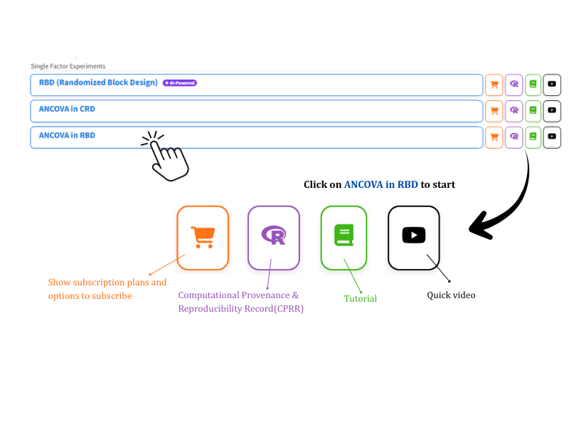
Now that the theory is clear, let us run the analysis. Visit the RAISINS home page at www.raisins.live and go to Data Analysis. In this tutorial we use the ANCOVA (RBD) module, the two-way ANCOVA shown in Figure 1.
5.1 Computational Provenance & Reproducibility Record
CPRR (Computational Provenance & Reproducibility Record) provides a transparent and comprehensive record. Click on the icon shown in Figure 1 to access CPRR and know about the computational workflow performed during the analysis. The record for this module states the R version and the exact version of every package used, names the specific function behind each reported result. CPRR lists every default parameter and decision rule applied by the module and provides fully runnable R code that reproduces each analytical step. Users can execute the code in R to independently reproduce and verify the results. It carries its own DOI.
To cite the platform itself in a paper, thesis, or report, use the RAISINS citation, available in APA, Harvard, and BibTeX formats at www.raisins.live/citation.html. That is the primary reference, and for most manuscripts it is all you need.
The CPRR for the ANCOVA (RBD) module is at www.raisins.live/module_record/ancova_rbd.html.
Cite the RAISINS paper as your primary reference for the platform. Add the CPRR as supporting documentation when a journal asks for details of the computing environment, or when you want your methods section to be precise about versions and functions rather than saying “analysis was carried out using an online tool.” The CPRR supports the citation and ensures computational reproducibility.
6 Preview Mode and Quick Tour
Before subscribing, you can explore the entire module using Preview mode, accessible from the Welcome page. Preview mode loads a built-in mango dataset so you can try every feature (the ANCOVA table, adjusted means with letter groupings, pairwise comparisons, the multivariate PCA index, residual normality checks, the basic and advanced plots, and the RA-One assistant) without uploading your own data. First-time users are also offered a Quick Tour, an interactive, step-by-step walkthrough that highlights each control and explains what it does. You can retake the tour at any time from the Quick Tour tab.
7 A Working Example
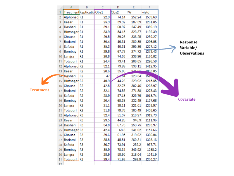
The rest of this tutorial follows one dataset: a mango variety trial. Ten treatments (the varieties Alphonso, Badami, Bombay, Chausa, Dasheri, Himsagar, Kesar, Langra, Safeda, and Totapuri) were grown in a Randomized Block Design with three replications each, giving 30 experimental units. For every unit, three response characters were recorded, Obs1, FW (fruit weight), and yield, and a fourth continuous measurement, Obs2, was recorded to serve as the covariate. Because the covariate is expected to influence the response, comparing the varieties on their raw averages could be misleading; ANCOVA adjusts each variety’s mean to a common covariate value before comparing them. The task the module settles is: once the covariate is accounted for, do the ten varieties genuinely differ in Obs1, FW, and yield?
8 Preparing Your Data
Your analysis is only as good as your data. Feed RAISINS high-quality data and it will deliver powerful insights; feed it messy data and the results will not be trustworthy. You have Four routes:
- Create your dataset in MS Excel
- Build your dataset directly within the RAISINS app
- Using the Model datasets in RAISINS as a reference
- Create your dataset using the RA-One chat assistant
8.1 Preparing Data in MS Excel
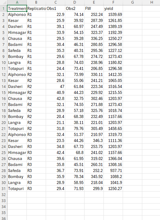
Open a new blank sheet in MS Excel containing only one sheet, and avoid adding any unnecessary content. The dataset should follow a column-based format. The first column holds the Treatment label (the ten varieties), the second holds the Replication (block) label, and one column holds the continuous covariate (here Obs2). All response characters under study (Obs1, FW, yield) then occupy separate columns. Each treatment label repeats once per replication, so with ten treatments and three replications every variety name appears three times. The file can be saved as CSV, XLS, or XLSX, but CSV is recommended as it is lighter and loads faster. Ensure there are no unwanted spaces in column names or labels. For reference, see the structure in Figure 3.
Dataset creation rules
- Column naming convention
- No spaces allowed in column names.
- Use underscores (
_) or full stops (.) for separation. - Avoid symbols and special characters such as %, #.
- Data arrangement
- Start the data towards the upper-left corner.
- Ensure the row above the data is not blank.
- Cell management
- Avoid typing or deleting in cells without data.
- If needed, select the affected cells, right-click, and choose Clear Contents.
- Column relevance
- Name all columns meaningfully.
- Exclude unnecessary columns not required for the analysis.
- Treatment, block, and covariate columns
- The Treatment column must contain the distinct treatment labels, each repeated once per replication.
- The Replication column must identify the block for every row, so that each treatment appears once in each block.
- The covariate must be a continuous numeric column, with a value for every row and no blanks.
How to save as CSV in MS Excel
Open your workbook. Ensure your data is arranged properly with only one sheet.
Click the ‘File’ menu. Go to the top-left corner and click File.
Choose ‘Save As’ or ‘Save a Copy’. Select the location where you want to save your file.
Set file type to CSV. In the ‘Save as type’ dropdown, choose CSV (Comma delimited) (*.csv).
Name your file. Enter a relevant file name without spaces (use underscores if needed).
Click ‘Save’. Click Save to export the file.
💡 Tip: Before saving, double-check that your data is on the first sheet and follows the required format: no empty rows above the data, meaningful column names, and a complete numeric covariate column.
8.2 Prepare Using Create Data in RAISINS
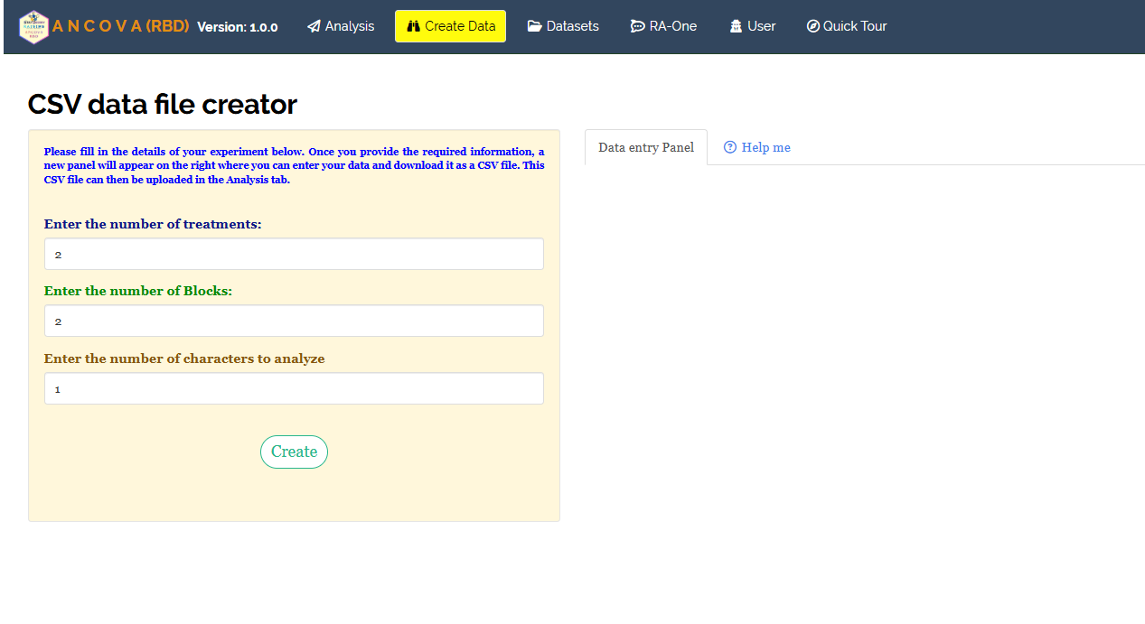
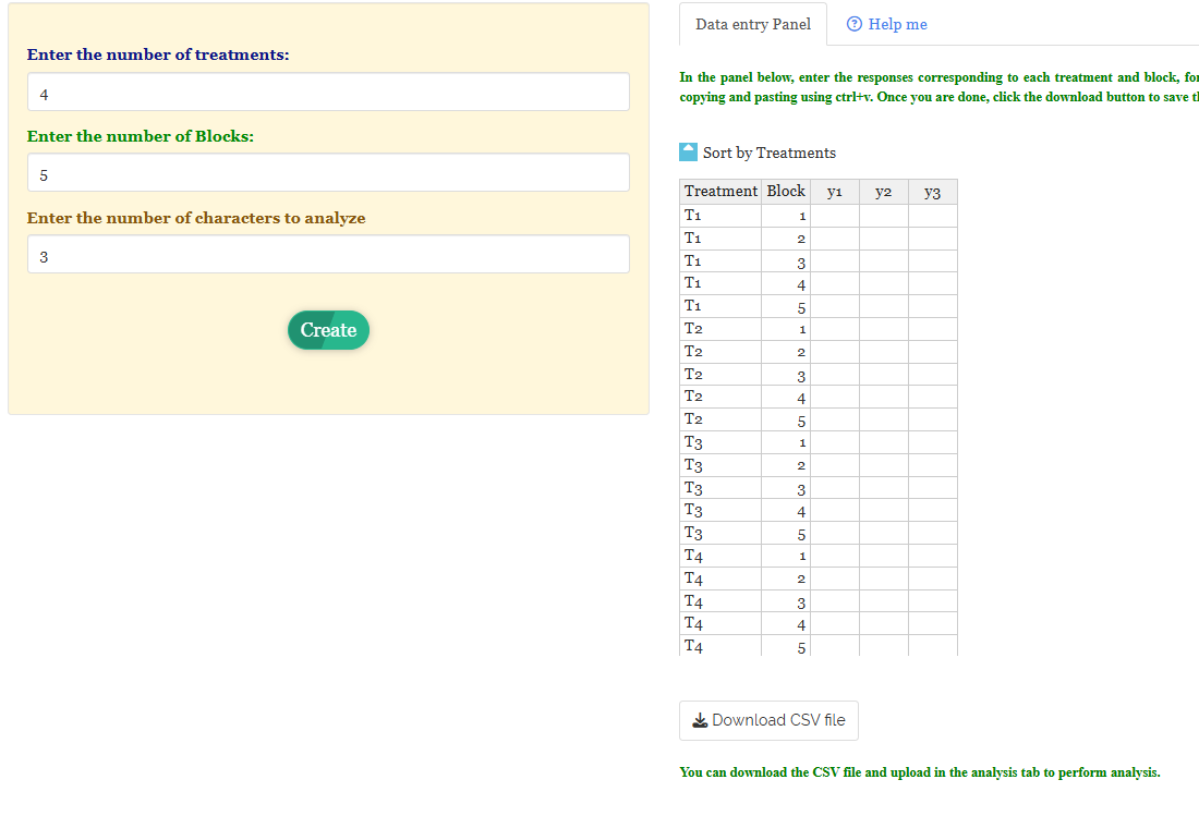
If you are unsure about the correct format, do not worry, RAISINS can create the data layout for you using the prescribed template. Open the Create Data tab (Figure 4 (a)) and:
- Enter the number of treatments
- Enter the number of Blocks (replications)
- Enter the number of characters to analyze
- Click the Create button
A ready-made data-entry panel appears on the right (Figure 4 (b)) with the Treatment and Block columns already filled in, and empty columns for each response character. You may type the observations straight into the panel or paste them from Excel with Ctrl+V. Once the values are entered, click Download CSV file and upload it under the Analysis tab.
8.3 Download Model Datasets
If you are unsure about the required data format or would like to explore the module before using your own data, RAISINS provides model datasets for reference. To download them:
- Navigate to the Datasets tab
- Click the Download CSV link corresponding to the required dataset
- Save the file to your computer
- Use the model dataset as a reference for preparing your own data or upload it directly to explore the analysis

8.4 Creating a Dataset Using RA-One Chat
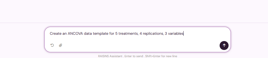
RA-One, the built-in chat assistant, can help you create a properly formatted dataset through a simple conversation. To get started, open the RA-One chat by clicking the chat icon available within the app or by heading over to the RA-One tab. Now you simply describe the design in plain language, for example “Create an ANCOVA data template for 5 treatments, 4 replications, 3 variables” (Figure 6), and RA-One generates a Two-Way ANCOVA (RBD) data-entry template with the Treatment and Block columns pre-filled and empty columns for the covariate and each response (Figure 7). You can enter or paste your values, download the template as a CSV file, and upload it directly under the Analysis tab. The full workflow is illustrated in Figure 7 below.
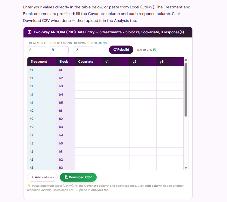
RA-One chat workflow: describe the design, generate the template, fill it in, and download the CSV
9 The Analysis Tab
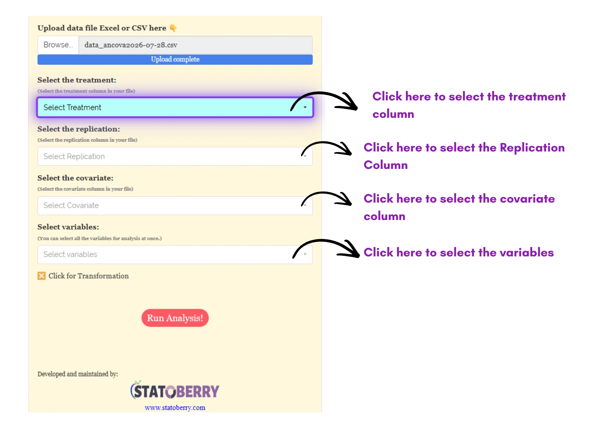
Figure 8 shows the sidebar of the Analysis tab, where the whole model is specified. Upload your prepared file by clicking Browse; once the upload completes, four selectors appear, and this is the step that defines a two-way ANCOVA:
- Select the treatment — choose the column holding your treatment labels (here Treatment, the ten varieties).
- Select the replication — choose the block column (here Replication). This is what makes the design an RBD rather than a completely randomized one.
- Select the covariate — choose the continuous column to adjust for (here Obs2). This is the defining ingredient of ANCOVA; without it you would be running a plain two-way ANOVA.
- Select variables — choose one or more response characters to analyse (here Obs1, FW, and yield). You can select them all at once, and RAISINS runs a separate ANCOVA for each.
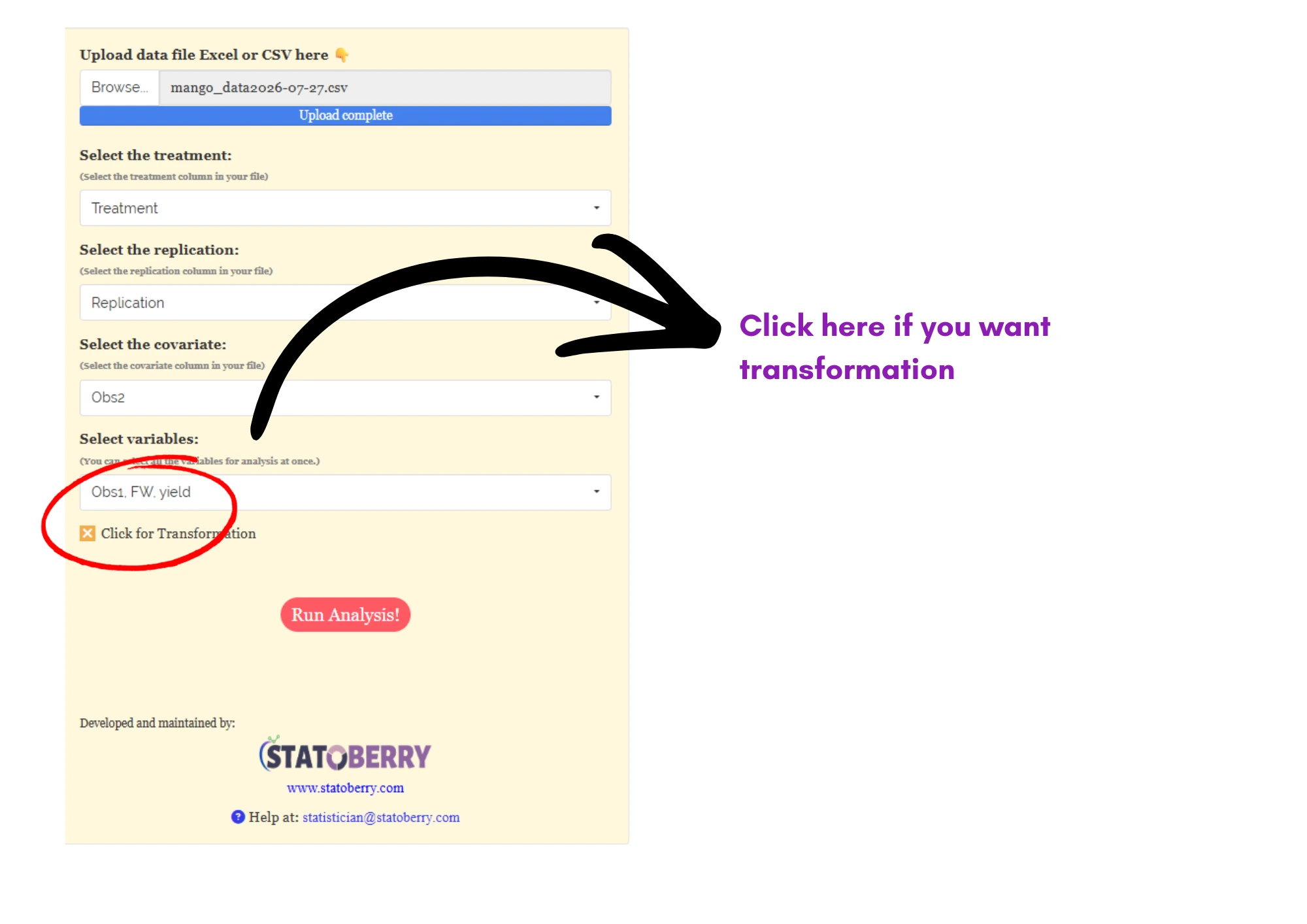
Below the selectors sits a Click for Transformation option (Section 10) for cases where the response needs to be transformed. When everything is set, click Run Analysis! and all outputs appear across the sub-tabs at the top of the page: Analysis.Results, Calculation, Basic Plots, Advanced Plots, Interpretation tab, Multivariate, FAQs, and View Data.
On the Analysis.Results panel itself, a control bar lets you tune the output without re-running anything: the Multiple comparison test used for the post-hoc pairwise stage (LSD by default), the P-adjustment applied to those comparisons (None by default), the Level of significance (α) (0.05 by default), the number of Digits after decimal, and the report Font. Adjust these to match your journal’s conventions.
The covariate (Obs2) and the response variables (Obs1, FW, yield) are different roles. The covariate is the background variable you want to remove; the responses are the characters you want to compare across varieties. Put the wrong column in the covariate slot and the adjustment corrects for the wrong thing. If you have no covariate to adjust for, this is the wrong module — use the ordinary two-way ANOVA (RBD) instead.
10 Transformation
If the residual normality check (Section 13) shows a clear departure, or the variance is obviously uneven, a transformation of the response can help. Tick Click for Transformation in the sidebar (Figure 9) and choose the transformation that suits your data. Log, square-root, and arcsine transformations are the common choices.
Logarithmic transformation converts a skewed distribution into a more symmetrical one by replacing each data point (x) with its logarithm. It is applied to positive, continuous data where the variance grows in proportion to the mean, a pattern common in phenomena that grow multiplicatively or exponentially.
Square root transformation stabilises variance and reduces right-skewness by replacing each data point (x) with its square root. It is primarily used for non-negative count data, such as those following a Poisson distribution, where variance increases with the mean. By compressing the upper end of the scale more than the lower end, it brings the data closer to normality.
Arcsine transformation (the angular transformation) is designed for proportions or percentages bounded between 0 and 1. By taking the inverse sine of the square root of the proportion, it stretches the ends of the distribution near 0 and 1, where variance is naturally small. It is chiefly used to achieve homoscedasticity in binomial data.
After choosing the appropriate transformation, proceed to Section 11 for the analysis.
11 Analysis Results
Once your dataset is uploaded and you click Run Analysis!, the two-way ANCOVA is performed for every selected character. The Analysis.Results sub-tab presents the output in two main tables that should be read in order: first the ANCOVA summary table, which tells you whether the treatments differ after adjustment, and then the adjusted-means table, which tells you which treatments differ. A separate Pairwise Comparison Table gives the full detail behind the letters. A short paragraph above the tables restates your design, here, ten treatments, three replications per treatment, and LSD chosen for the post-hoc comparison at α = 0.05.
Table 1: ANCOVA summary (mean squares and significance)
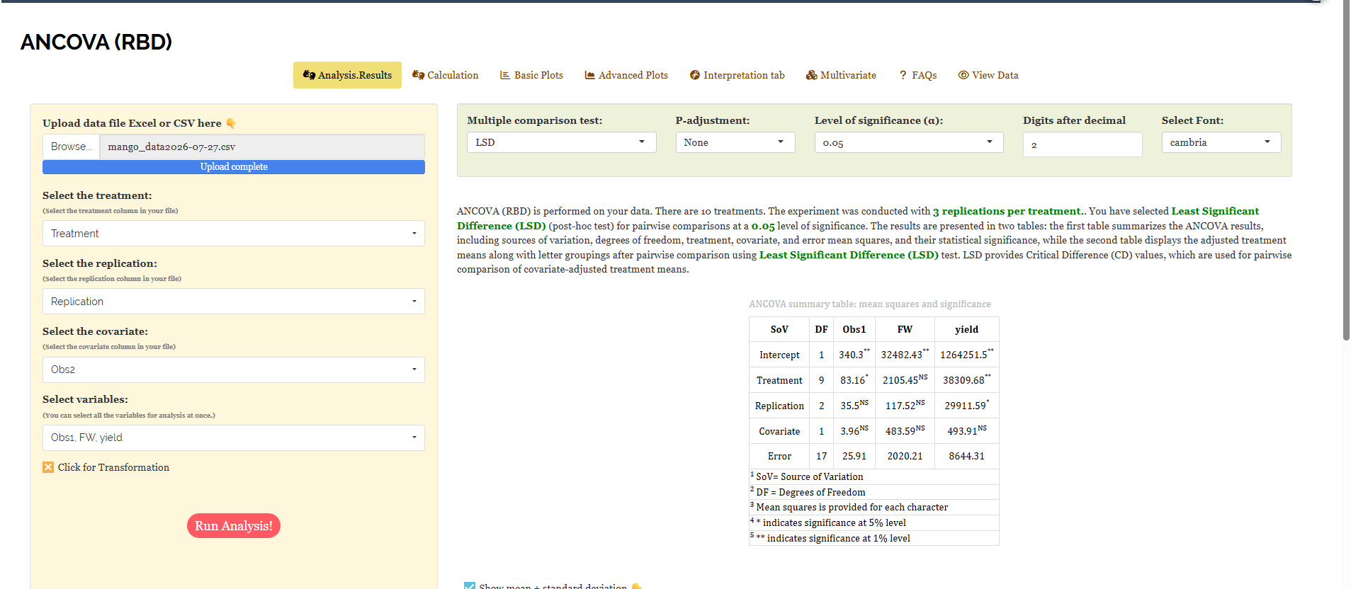
Each row is a source of variation (SoV), and each response column reports that source’s mean square, with asterisks marking significance. Reading Figure 10 for the working example:
- Treatment — for Obs1 the treatment mean square is 83.16, significant at the 5% level ( * ); for yield it is 38309.68, significant at the 1% level ( ** ); for FW it is 2105.45 and non-significant (NS). So the varieties differ for Obs1 and yield, but not for fruit weight.
- Replication — significant only for yield (29911.59, * ), confirming that blocking removed real field variation for that character, exactly the benefit an RBD is meant to provide.
- Covariate (Obs2) — non-significant for all three characters (Obs1 3.96 NS, FW 483.59 NS, yield 493.91 NS). In this dataset the covariate did not explain much variation, so the adjusted means will sit close to the raw ones. As noted in Section 1, that is a perfectly good outcome, not a reason to drop the covariate.
- Error — the leftover mean square (Obs1 25.91, FW 2020.21, yield 8644.31) on 17 degrees of freedom, the yardstick every treatment F-test is measured against.
How this table is built
Each source’s sum of squares is computed adjusted for the others, so the treatment effect is judged after the block and covariate contributions have been removed. Dividing a source’s sum of squares by its degrees of freedom gives its mean square, and dividing that by the error mean square gives its F-statistic, which is converted to a p-value. The degrees of freedom follow the design: treatment = (t − 1) = 9, replication = (r − 1) = 2, covariate = 1 for the single slope, and error = 17, which is what remains of the 29 total degrees of freedom (30 units minus 1). Significance is marked with a single asterisk ( * ) at the 5% level and two asterisks ( ** ) at the 1% level, with NS for non-significant.
Table 2: Adjusted (estimated marginal) means with letter groupings
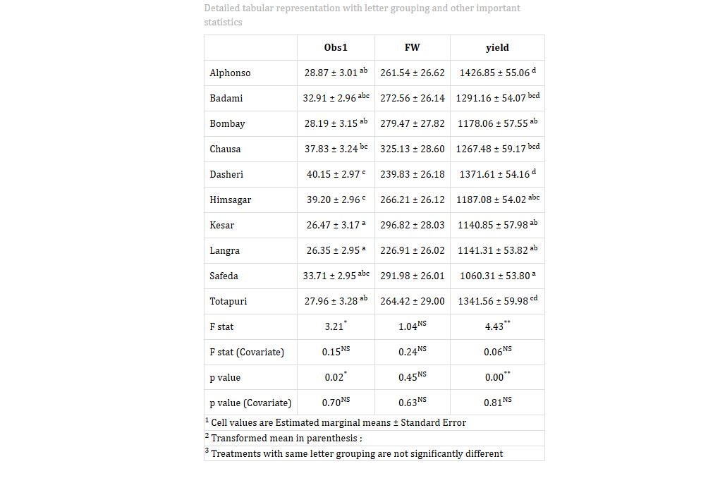
This is the table you report. Each cell is a treatment’s estimated marginal mean ± standard error, that is, the covariate-adjusted mean, followed by a letter grouping from the LSD post-hoc test. The rule for reading letters is simple: treatments that share at least one letter are not significantly different; treatments with no letter in common are. The footer also gives the overall F stat and p value for the character, and a separate F stat (Covariate) and p value (Covariate) so you can see the covariate’s contribution at a glance.
For Obs1 (F = 3.21, p = 0.02), Dasheri has the highest adjusted mean (40.15 ± 2.97, group c) and Langra the lowest (26.35 ± 2.95, group a); because Dasheri carries c and Langra carries a with no shared letter, the two differ significantly, while Dasheri, Himsagar (39.20, c) and Chausa (37.83, bc) share letters and are statistically on par. For yield (F = 4.43, p = 0.00) Alphonso is highest (1426.85 ± 55.06, group d) and Safeda lowest (1060.31 ± 53.80, group a). For FW the character was non-significant (F = 1.04, p = 0.45), so no meaningful separation among varieties is claimed. Note the F stat (Covariate) values (0.15, 0.24, 0.06) and their large p-values (0.70, 0.63, 0.81), the numeric confirmation that Obs2 did not materially shift the comparison here.
Table 3: Pairwise comparison table
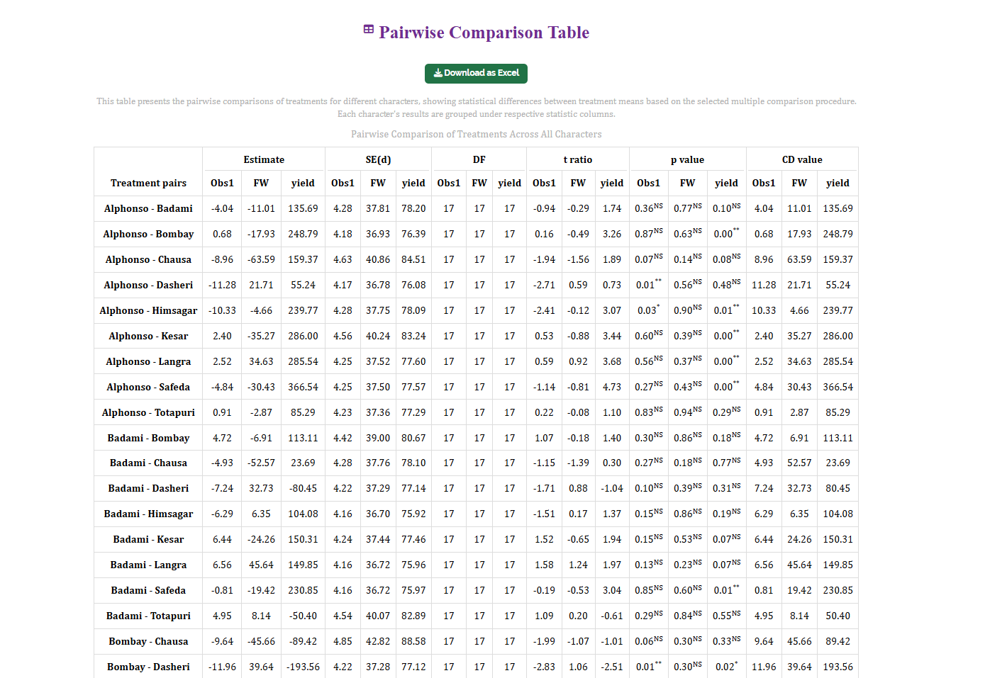
The letter groupings in Figure 11 are a compact summary of the full set of pairwise comparisons, and Figure 12 is that full set. For every pair of treatments and every character, RAISINS reports the Estimate (the difference between the two adjusted means), the SE(d) (standard error of that difference), the DF (17 throughout, the error degrees of freedom), the t ratio, the p value, and the CD value (Critical Difference, the smallest difference that would be significant at α). For example, the Alphonso–Dasheri difference in Obs1 is −11.28 with t = −2.71 and p = 0.01 ( ** ), a significant gap, which is why Alphonso and Dasheri do not share a letter for Obs1 in Figure 11. Two treatments are significantly different whenever the absolute Estimate exceeds the CD value, equivalently whenever the p-value is below α.
A tiny difference can be statistically significant if your trial is large or tightly controlled, and an agronomically valuable difference can miss significance in a small trial. Always read the size of the adjusted mean difference against the CD value and ask whether a gap of that magnitude matters in the field, not just on the page. And remember that a non-significant character (FW here) means no evidence of a difference, which is not the same as proof that the varieties are identical.
12 Multivariate: PCA-Based Index
The three characters were analysed one at a time above, but you often want to rank the varieties on all characters together. The Multivariate sub-tab offers a Principal Component Analysis (PCA) based index for exactly this. PCA reduces the several characters into a smaller set of uncorrelated principal components that capture the shared pattern, and a PCA-based index score then lets you select or rank treatments on all characters collectively. Click Click here for PCA Index to compute it (Figure 13).
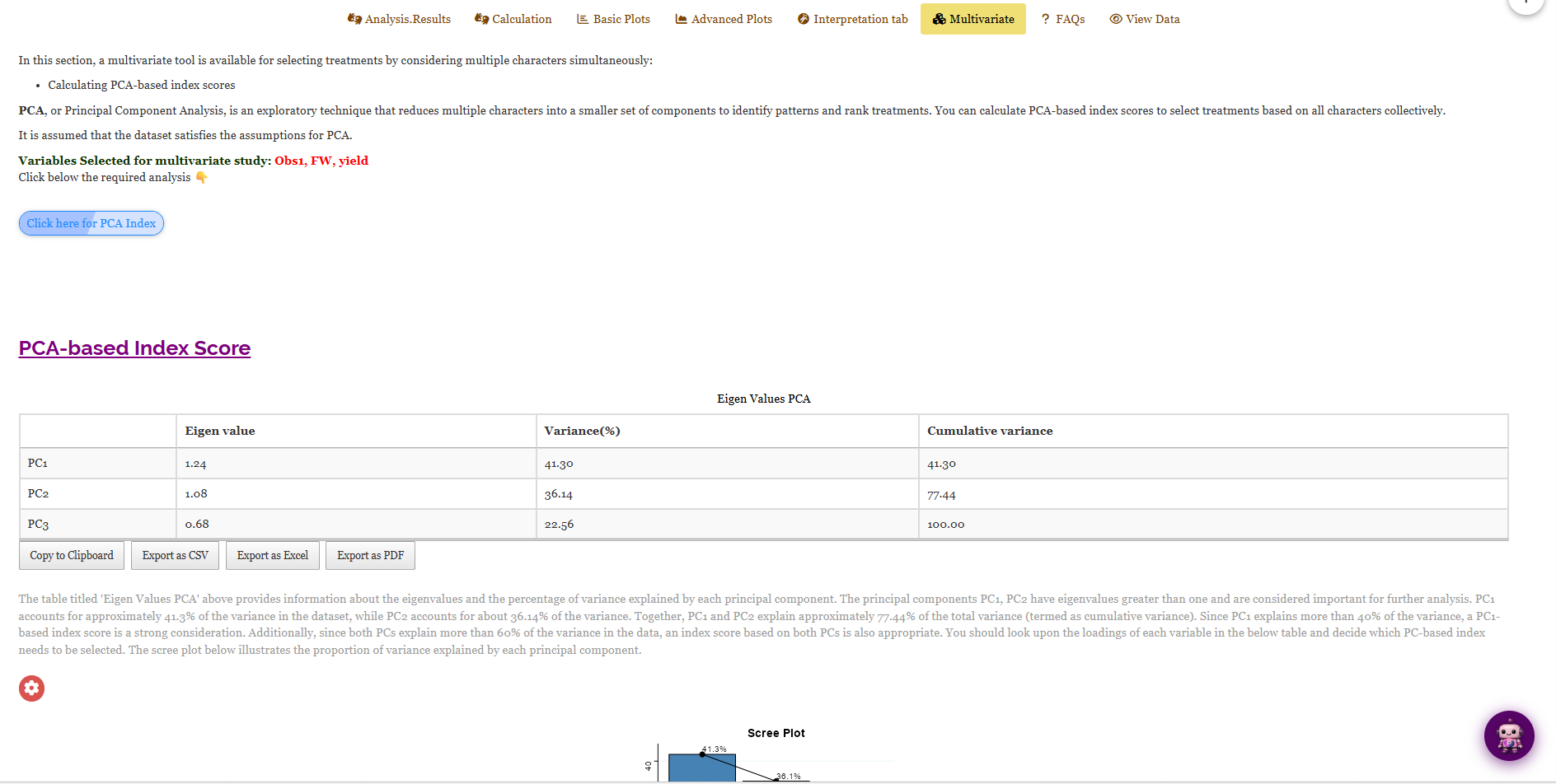
The Eigen Values PCA table reports, for each component, its eigenvalue, the percentage of variance it explains, and the cumulative variance. In the working example PC1 has an eigenvalue of 1.24 and explains 41.30% of the variation, PC2 has an eigenvalue of 1.08 explaining 36.14%, and together they account for 77.44% of the total (PC3 contributes the remaining 22.56%). Components with an eigenvalue above 1 are the ones worth retaining, so both PC1 and PC2 are meaningful here; since PC1 alone explains more than 40% and the two together exceed 60%, an index built on PC1, or on PC1 and PC2 combined, is a sound basis for ranking the varieties across all three characters at once. The scree plot beneath the table shows the same information visually.
The single-character ANCOVA answers “which variety is best for yield?” The PCA index answers “which variety is best overall, weighing Obs1, FW and yield together?” Use it when no single character is decisive and you need one combined ranking, but check the variable loadings (shown below the table in the app) so you know which characters each component is really rewarding.
13 Normality Check and Plots
Why check residuals rather than the raw data?
-
ANCOVA assumes that the residuals of the fitted model, what is left of each observation after the treatment, block, and covariate effects are removed, are approximately normally distributed. This is subtly different from the t-test, which checks normality within each group: because ANCOVA has already accounted for several sources of structure, it is the model’s leftovers, not the raw response, that should look normal. A residual QQ plot is therefore the natural diagnostic. For larger trials the analysis is fairly robust to mild departures, but a clear curve or heavy tails is worth acting on with a transformation (Section 10).
The Advanced Plots sub-tab provides a QQ Plot that checks residual normality directly (Figure 14). It ranks the ANCOVA model’s residuals and plots them against the values expected under a perfect normal distribution. If the assumption holds, the points fall close to the straight diagonal line.
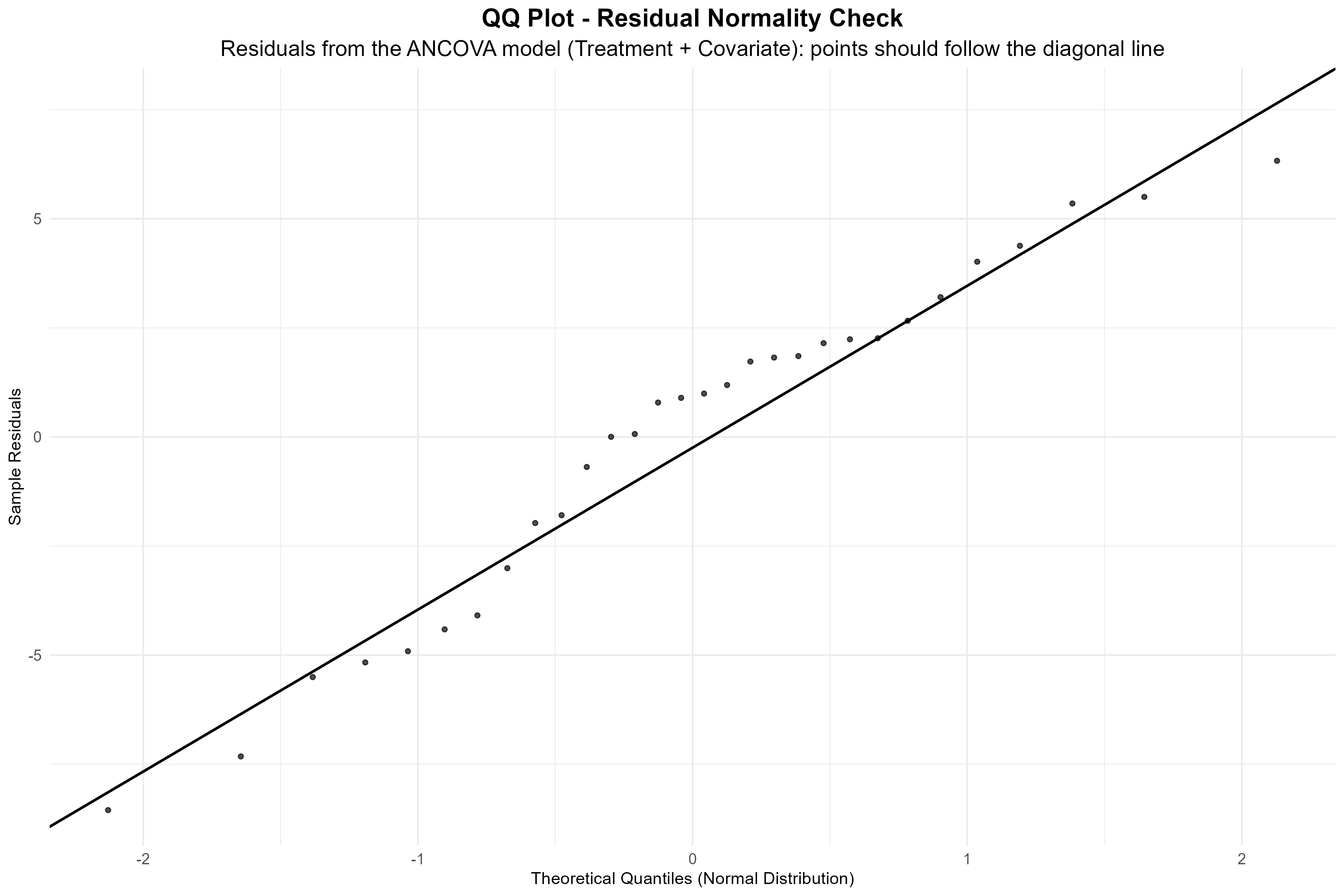
In Figure 14 the points hug the diagonal closely along its length, with only mild wandering at the extreme ends, the ordinary behaviour of a small sample and no cause for concern. A pronounced S-shape, a clear curve, or points flying away at both ends would instead signal a real departure from normality, at which point a log or square-root transformation (Section 10) is the usual remedy.
13.1 Basic Plots
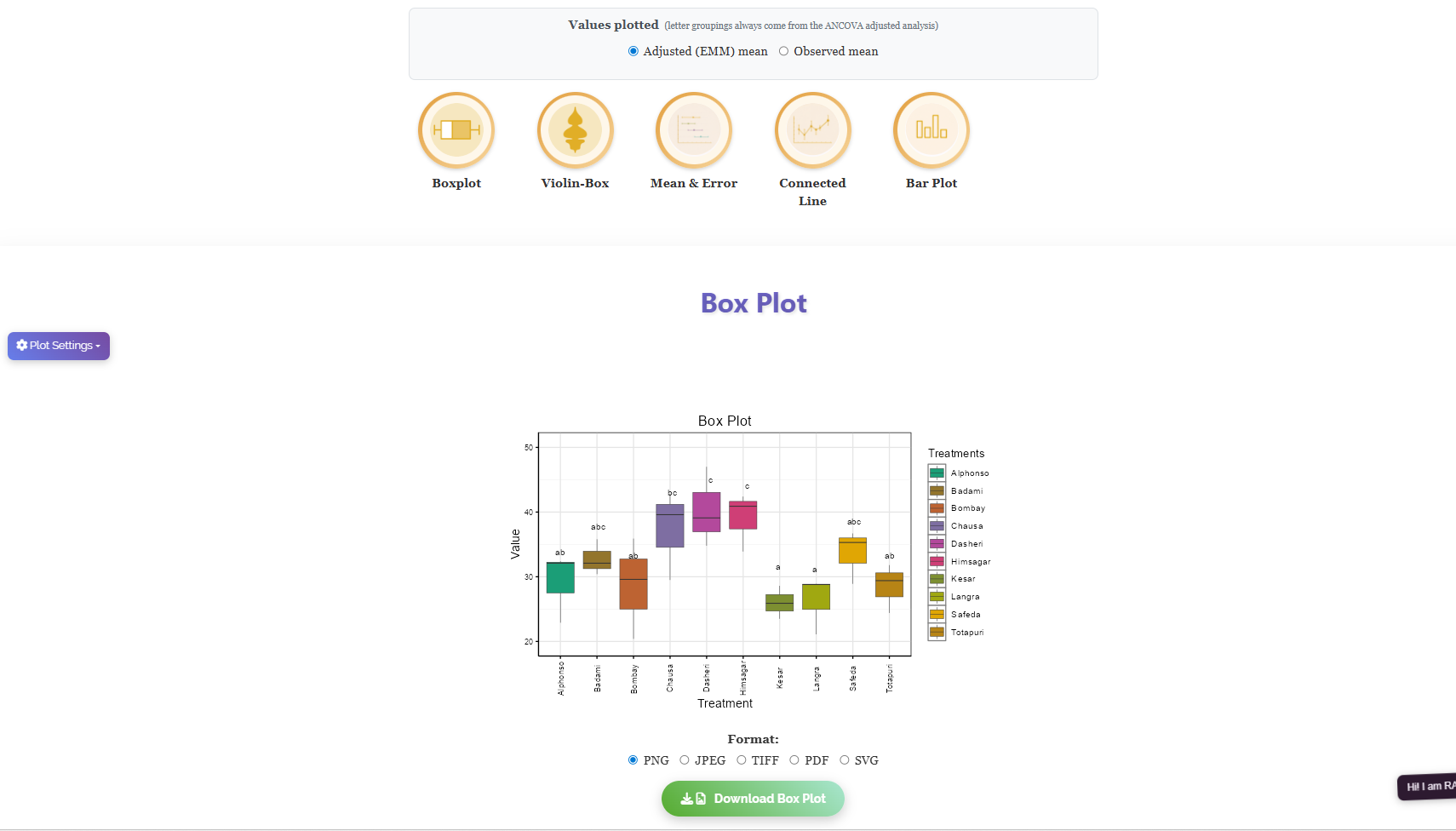
The Basic Plots sub-tab turns the adjusted means into publication-ready graphics. Five plot styles are available, Boxplot, Violin-Box, Mean & Error, Connected Line, and Bar Plot, and a toggle at the top lets you plot either the Adjusted (EMM) mean or the Observed mean. Whichever you choose, the letter groupings always come from the ANCOVA adjusted analysis, so the significance letters stay consistent with Figure 11. Each plot is fully customisable through Plot Settings and can be downloaded as PNG, JPEG, TIFF, PDF, or SVG. Figure 15 shows the boxplot view.
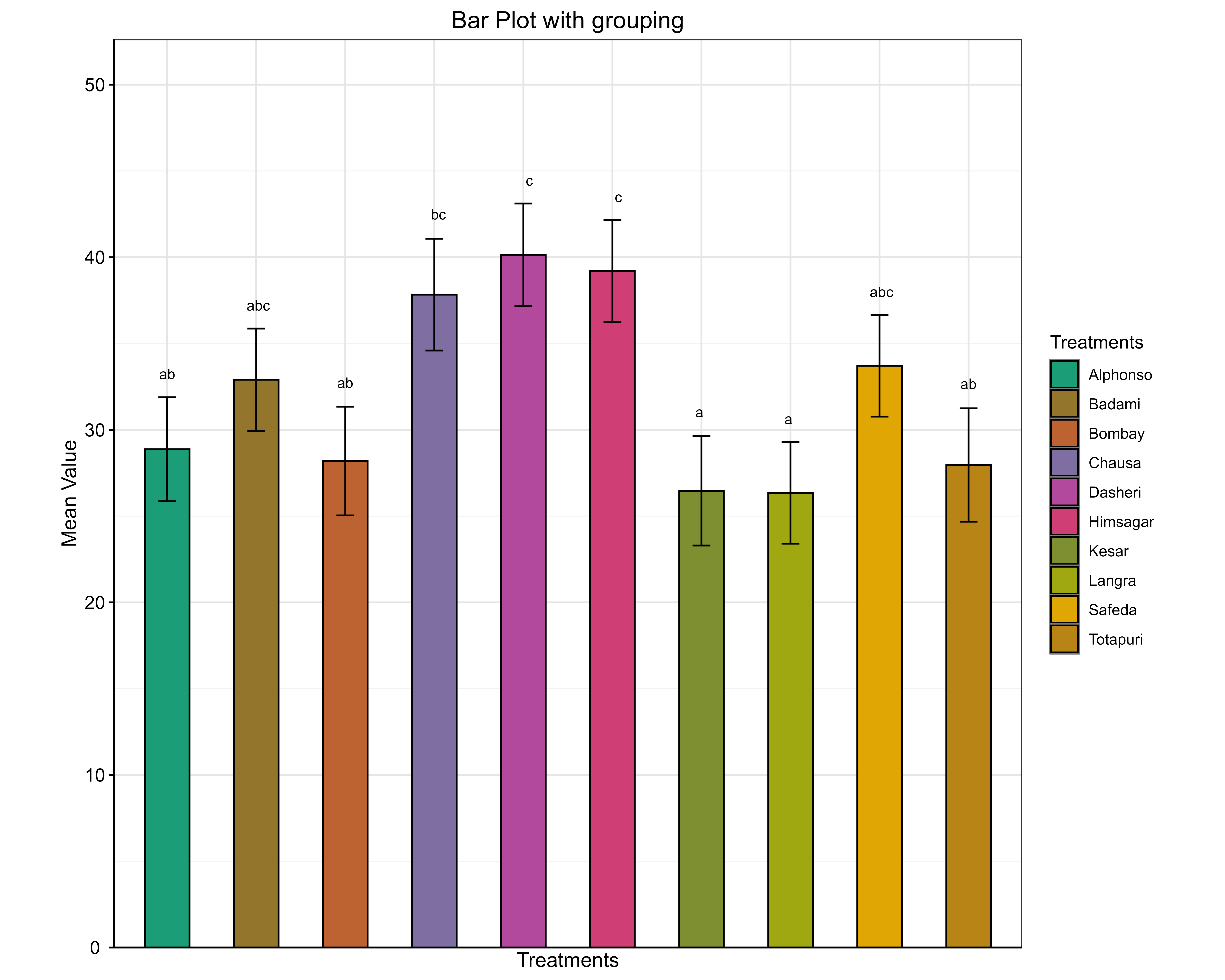
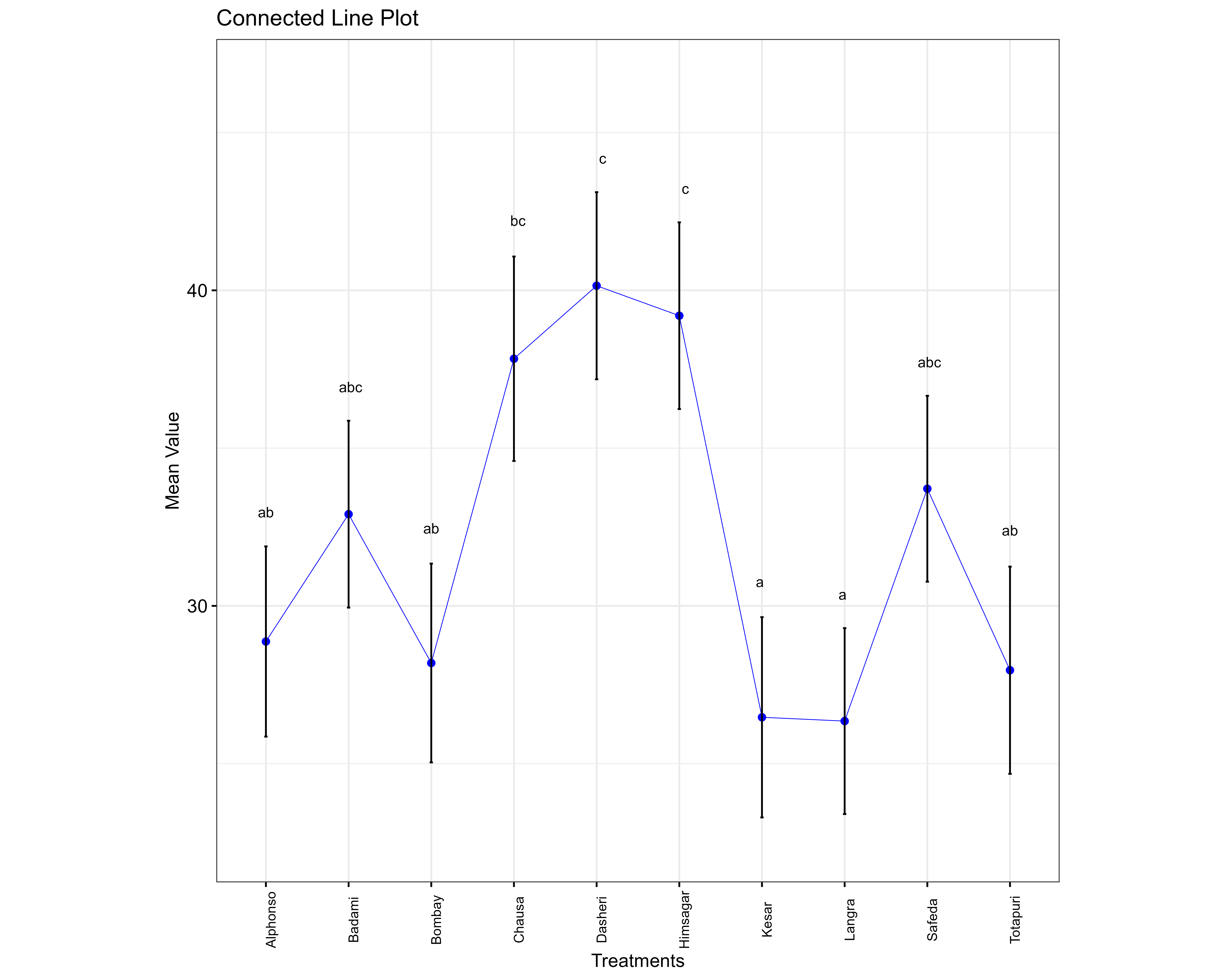
The Bar Plot (Figure 16 (a)) presents each variety’s adjusted mean as a bar with an error bar and its letter group printed above, while the Connected Line plot (Figure 16 (b)) joins the adjusted means so peaks and troughs across varieties stand out at a glance. Both carry the same a/b/c letters as the results table, so the graphic and the statistics always agree.
13.2 Advanced Plots
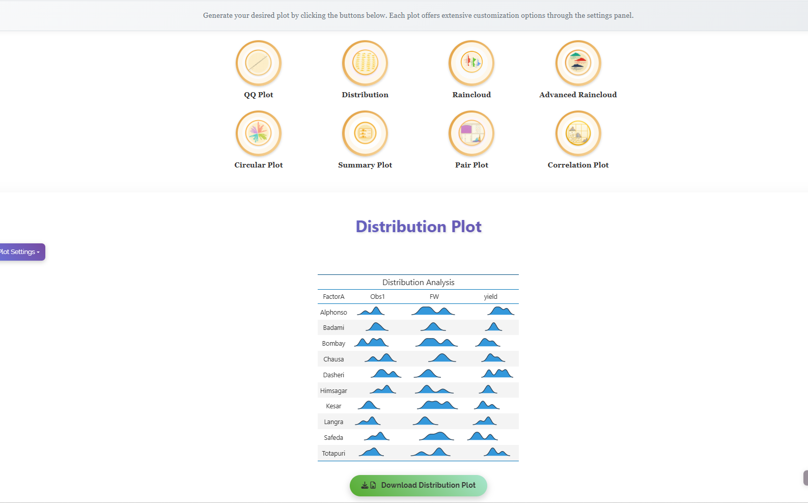
The Advanced Plots sub-tab goes beyond the summary graphics to help you inspect the data’s shape and relationships. Alongside the residual QQ Plot already discussed, it offers a Distribution view, Raincloud and Advanced Raincloud plots, a Circular Plot, a Summary Plot, a Pair Plot, and a Correlation Plot (Figure 17). These are exploratory tools: use them to spot skewness, outliers, and how the characters relate to one another before you finalise the analysis.
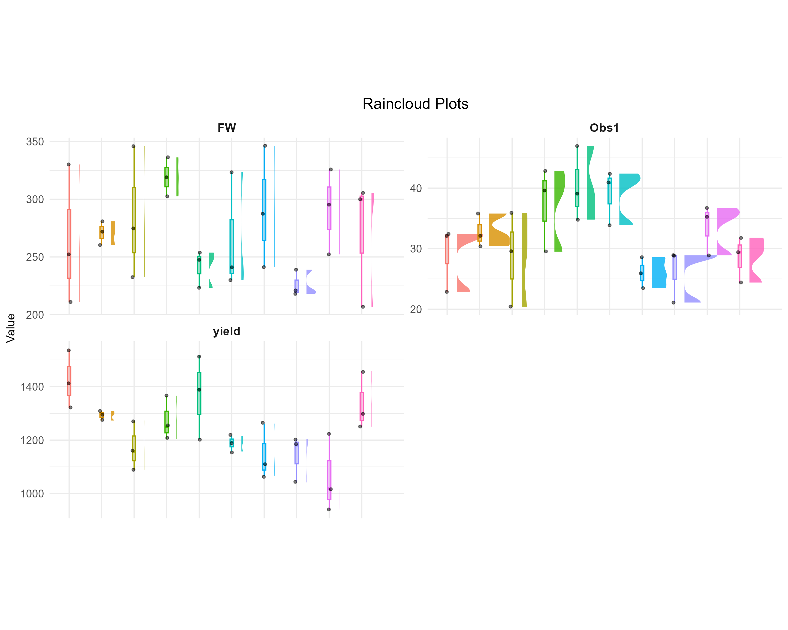
The Raincloud plot (Figure 18) is particularly useful in a small trial: for each character it combines a box plot, the individual data points (“rain”), and a smoothed density (“cloud”), so you can see the spread and the raw observations together rather than trusting a single summary statistic.
14 Interpretation
RAISINS provides a clear, ready-to-use interpretation of your results in plain English. Tick the confirmation box (which also asks you to confirm the analysis ran without error) and click Click here for interpretation. The assistant restates the design, a Two-Way ANCOVA (RBD) with ten treatments and three replications, names the characters that showed significant treatment differences, explains the LSD letter groupings, and points out the highest and lowest varieties for each significant character. You can access this from the Interpretation tab (Figure 19).
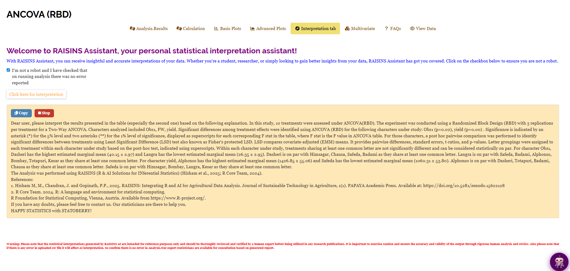
For the working example the interpretation confirms exactly what the tables showed: treatment effects were significant for Obs1 (p = 0.02) and yield (p = 0.00) but not for FW; Dasheri had the highest adjusted mean for Obs1 (40.15 ± 2.97) and Langra the lowest (26.35 ± 2.95); Alphonso had the highest yield (1426.85 ± 55.06) and Safeda the lowest (1060.31 ± 53.80). It closes with the RAISINS citation for your methods section.
The generated text is a drafting aid, not a substitute for your judgement. As the module itself warns, an error in the uploaded file will carry through into the interpretation, so confirm the analysis ran cleanly first, and have a human expert verify the wording before it goes into a publication.
15 Chat with Your Data Using RA-One
RA-One is the built-in conversational assistant for the ANCOVA (RBD) module, available from the RA-One tab. You ask questions in plain language and it answers using your own analysis rather than generic statistical advice. Every result it discusses is drawn from what the module actually computed - it never invents numbers, and if a value isn’t available it says so instead of guessing. All answers are in plain English, with no code or software commands.
RA-One works directly with your ANCOVA table, adjusted means, pairwise comparisons, and interpretation outputs. It can explain what an adjusted (estimated marginal) mean is for your specific varieties, tell you why two treatments do or do not share a letter, clarify what the non-significant covariate means for your conclusions, and answer general concept questions such as how the Critical Difference is used or why blocking matters. When you open the tab it greets you with quick-start cards, Interpret results, Create data template, Model datasets, and Report results, so you can jump straight to a task (Figure 20).
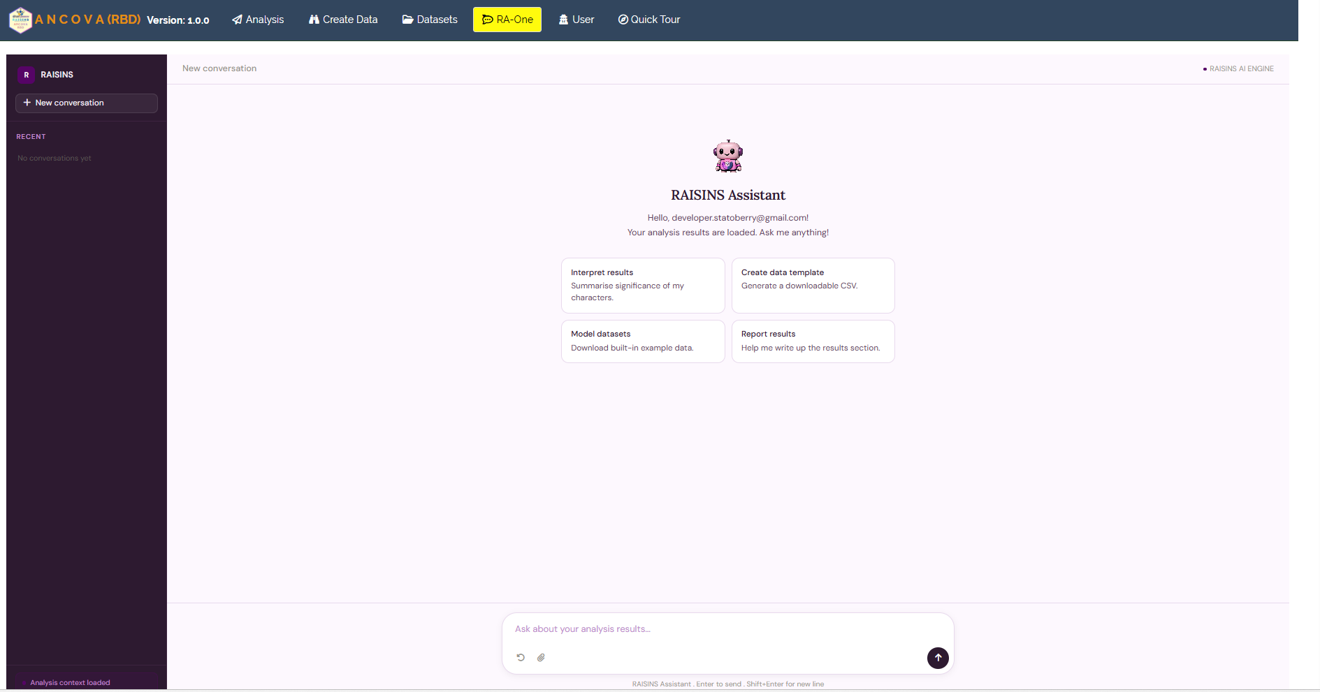
The same chat window can also prepare your data. It can build a correctly formatted dataset template (Section 8.4) for you to fill in, or fetch a model dataset (Section 8.3) so you can try the module straight away - so you never need to leave the tab to get a file ready.
RA-One can also generate plots on request. Ask for a bar plot or connected-line plot of the adjusted means, a raincloud plot for a character, or the residual QQ plot, and the app renders the graphic directly in the chat, where you can view it and refine it by asking for changes (Figure 21).

Within a single conversation, RA-One can interpret your results, build a data template, fetch a model dataset, and produce plots - so most of a routine ANCOVA session can be conducted without ever leaving the chat window.
16 FAQs
The module includes a dedicated FAQs section to clarify common doubts and guide you through the features. It offers detailed answers, additional information, and helpful tips for a smooth experience. If you are ever unsure how something works, say what to do when the covariate turns out non-significant, how to read the letter groupings, or the difference between the adjusted and observed means, the FAQs are a good place to start.
17 View Data
View Data is the primary diagnostic tool for ensuring data integrity before analysis. When you upload your dataset, the system performs an automated Health Check to validate column types and formatting. For a two-way ANCOVA this step is especially important: it confirms that the Treatment and Replication columns are read as grouping factors, that the covariate and every response column are numeric, that each treatment appears once in every block, and that there are no missing or badly formatted entries that could distort the adjustment.
18 Wrapping Up
The two-way ANCOVA rests on one honest question: once every plot is placed on an equal footing for the covariate, and the blocks are accounted for, do the treatment means still differ? Everything else, the RBD structure, the covariate adjustment, the LSD letter groupings, the residual checks, exists only to make sure that question is answered fairly. RAISINS automates the machinery so you can concentrate on what the answer means for your research.
If your design does not fit this module, the companion modules are there: the ordinary two-way ANOVA (RBD) when there is no covariate to adjust for, the one-way ANCOVA (CRD) when your trial is completely randomized rather than blocked, and the regression module when you care about the covariate relationship itself rather than treatment comparison. And if you get stuck at any point, RA-One is available 24 × 7, or write to us at [email protected].
