Two-Factor Factorial CRD
A two-factor factorial CRD tests two factors and their interaction on homogeneous experimental units. This tutorial explains where the design is used, how to size it, how main effects and interaction are defined, and how to run the whole analysis in RAISINS… Read more …
A two-factor factorial experiment examines two factors simultaneously, estimating the main effect of each and, importantly, their interaction, that is, whether the effect of one factor depends on the level of the other. Laid out in a Completely Randomized Design (CRD), it suits experiments with homogeneous experimental material, such as pot-culture, laboratory and growth-chamber studies. RAISINS performs the complete analysis; factorial ANOVA, post-hoc mean comparisons, effect sizes, assumption diagnostics and multivariate follow-ups, without any programming. The sections that follow describe the procedure step by step.
1 What is a two-factor factorial design?
Consider an agronomist who wishes to improve crop yield, where yield depends on two factors: the variety sown and the fertilizer applied. Suppose two varieties, a and b, and three fertilizers, A, B and C, are under study. One approach is to vary a single factor at a time, holding the other fixed. This is inefficient and incomplete: neither experiment estimates both effects, and neither can reveal whether one variety responds better to a particular fertilizer than another does.
A factorial experiment avoids this limitation by combining every level of one factor with every level of the other. Here this gives \(2 \times 3 = 6\) treatment combinations,
\[ aA,\; aB,\; aC,\; bA,\; bB,\; bC \]
each of which is grown and measured. A single experiment therefore yields estimates of the variety effect, the fertilizer effect, and the extent to which the two depend on each other.
Does the effect of one factor depend on the level of the other?
This dependence is the interaction effect. When the experimental units are uniform all treatment combinations can be allotted to the units completely at random. This layout, factorial treatments assigned by complete randomisation, is the two-factor factorial in a Completely Randomized Design (CRD) analysed in this module.
2 How many observations will you need?
To determine the total number of experimental units needed, Count the levels of each factor and the number of replications (how many times each combination is repeated):
- Let factor A have \(a\) levels and factor B have \(b\) levels.
- The number of distinct treatment combinations is the product
\[ a \times b \]
- If each combination is replicated \(r\) times, the total number of observations is
\[ N = a \times b \times r \]
For example, the working dataset used later in this tutorial has \(a = 6\) levels of Factor A, \(b = 3\) levels of Factor B and \(r = 5\) replications, giving \(6 \times 3 = 18\) combinations and \(N = 6 \times 3 \times 5 = 90\) observations.
The replications are what give the analysis something to compare the treatment effects against, the error. In a two-factor factorial CRD the error degrees of freedom are
\[ df_{error} = a \, b \, (r - 1) \]
so that same \(6 \times 3 \times 5\) experiment carries \(18 \times (5 - 1) = 72\) error degrees of freedom, the figure you will see in the ANOVA table.
The F-tests in a factorial ANOVA are only powerful when the error has enough degrees of freedom. A common rule of thumb is to aim for at least 12 error degrees of freedom. Because \(df_{error} = ab(r-1)\), the lever you control is the number of replications \(r\), add replications rather than levels if the design feels thin. RAISINS’ template builder warns you when the error df drops below 12.
3 Creating your design template
Entering collected data systematically in an excel spreadsheet helps to reduce any chance for miscalculation, RAISINS builds this template for you in two ways: the Create Data tab and the RA-One chat assistant. Based on the levels of factors under study.
3.1 Route 1 - the Create Data tab
Open the Create Data tab and fill in four boxes (Figure 1):
- Levels of Factor A - how many levels the first factor has,
- Levels of Factor B - how many levels the second factor has,
- Number of Replications - how many times each combination is repeated,
- Number of characters to analyze - how many response variables (traits) you plan to measure.
Click Create, and the Data entry Panel on the right fills with every combination of Factor A and Factor B, each repeated for the requested replications, with response column (y1, y2, …) waiting for your data. Enter the values by hand, or paste a column straight from Excel. When the table is complete, click Download CSV file and upload it under the Analysis tab.
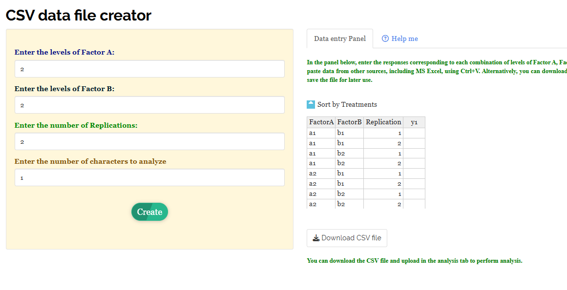
The tick-box above the entry panel controls the row order. Sorted by treatments, the rows are grouped so that all replications of a1 b1 sit together, then a1 b2, and so on, which is the easiest order to type into from a field book. The order of rows never affects the analysis; RAISINS reads the factor columns, not the row sequence.
3.2 Route 2 - the RA-One (AI) assistant
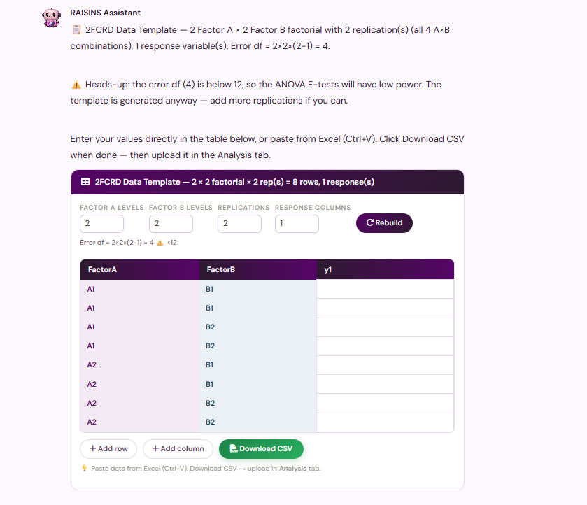
If you would rather just describe your experiment in words, ask RA-One. Tell it, for instance, “make a 2FCRD template with Factor A at 2 levels, Factor B at 2 levels, 2 replications and 1 response”, and it returns a ready-to-fill template (Figure 2).Ra-one also calculate the df using the levels of the factor and the number of replication
4 Calculation of Main effect and Interaction effect
To learn about the main effect and interaction effect, let us use a simple agricultural experiment with 2 factors, each at 2 levels. Consider an experiment in which the effect of fertilizer and irrigation on yield of a crop is studied. Factor A is fertilizer, at 50 kg/ha (low) and 100 kg/ha (high); factor B is irrigation, at 3 irrigations (low) and 6 irrigations (high). Suppose the crop yield observed under each treatment combination is given below:
| Combination | Fertilizer (A) | Irrigation (B) | Yield (t/ha) | Response symbol |
|---|---|---|---|---|
| both low | 50 kg/ha | 3 irrigations | 3.0 | \((1)\) |
| A high only | 100 kg/ha | 3 irrigations | 3.5 | \((a)\) |
| B high only | 50 kg/ha | 6 irrigations | 4.0 | \((b)\) |
| both high | 100 kg/ha | 6 irrigations | 6.0 | \((ab)\) |
Here \((1)\) is the yield when both factors are at their low levels, \((a)\) is the yield when fertilizer is high and irrigation is low, \((b)\) is the yield when fertilizer is low and irrigation is high, and \((ab)\) is the yield when both fertilizer and irrigation are at their high levels. These four responses will be used to calculate the main effects and interaction effect.
4.1 The main effect of a factor
Read Figure 3 along its edges. The bottom edge holds irrigation at 3 irrigations, so increasing fertilizer from 50 kg/ha to 100 kg/ha changes the yield from \((1)\) to \((a)\). The top edge holds irrigation at 6 irrigations, so the same increase in fertilizer changes the yield from \((b)\) to \((ab)\).
The main effect of a factor is the average change in the response when that factor moves from low to high, averaged over the levels of the other factor. Increasing fertilizer from 50 kg/ha to 100 kg/ha changes the yield by \((a)-(1)\) when irrigation is low, and by \((ab)-(b)\) when irrigation is high. Averaging these two changes gives the main effect of fertilizer (factor A):
\[A = \tfrac{1}{2}\big[(a)-(1) + (ab)-(b)\big]\]
or equivalently,
\[A = \tfrac{1}{2}\big[(ab) + (a) - (b) - (1)\big]\]
By the same reasoning, the main effect of irrigation (factor B) averages the change in yield from 3 irrigations to 6 irrigations across both fertilizer levels:
\[B = \tfrac{1}{2}\big[(b)-(1) + (ab)-(a)\big]\]
or equivalently,
\[B = \tfrac{1}{2}\big[(ab) + (b) - (a) - (1)\big]\]
4.2 The interaction effect
The interaction asks whether the effect of one factor depends on the level of the other. The effect of voltage when current is high is \((ab)-(a)\); when current is low it is \((b)-(1)\). If these two are equal, the factors act independently and there is no interaction. Their difference, halved, is the interaction effect:
\[ AB = \tfrac{1}{2}\big[(ab) + (1) - (a) - (b)\big] = \tfrac{1}{2}(a-1)(b-1) \]
please not that interaction of A with B is identical to the interaction of B with A.
A large interaction does not mean that the factors are more important. Instead, it means that the effect of one factor depends strongly on the level of the other factor, so the main effect of a single factor should not be interpreted in isolation. When the interaction effect (\(AB\)) is close to zero, the factors act more independently, and the main effects can be interpreted with greater confidence.
5 Getting to the module
Now let us run the analysis. Visit the RAISINS home page at www.raisins.live and open the Two factor experiment section under the Analysis of experiment section. Among the design and analysis tools, choose 2FCRD - Two factor factorial in CRD. Where you can upload your data, select the the two factor columns and the response columns, and it produces every table, plot and interpretation for you.
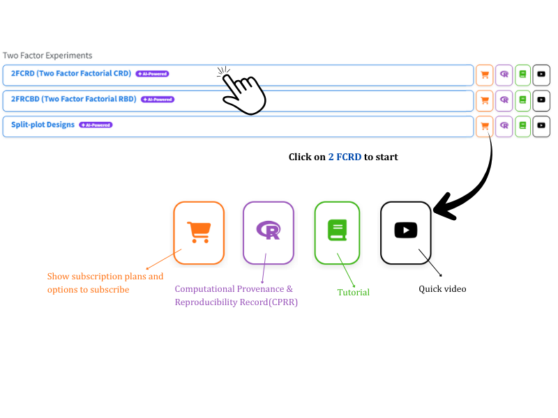
5.1 Computational Provenance & Reproducibility Record
CPRR (Computational Provenance & Reproducibility Record) provides a transparent and comprehensive record. Click the CPRR icon in the module header to see the exact computational workflow behind the analysis. The record for this module states the R version and the exact version of every package used, and names the specific function behind each reported result. CPRR lists every default parameter and decision rule applied by the module and provides fully runnable R code that reproduces each analytical step. Users can execute the code in R to independently reproduce and verify the results. It carries its own DOI.
To cite the platform itself in a paper, thesis, or report, use the RAISINS citation, available in APA, Harvard, and BibTeX formats at www.raisins.live/citation.html. That is the primary reference, and for most manuscripts it is all you need.
The CPRR for the two-factor factorial CRD module is at www.raisins.live/module_record/2FCRD.html.
Cite the RAISINS paper as your primary reference for the platform. Add the CPRR as supporting documentation when a journal asks for details of the computing environment, or when you want your methods section to be precise about versions and functions rather than saying “analysis was carried out using an online tool.” The CPRR supports the citation and ensures computational reproducibility.
6 Preview mode and Quick Tour
Before subscribing, you can explore the entire module using Preview mode, accessible from the Welcome page. Preview mode loads a built-in factorial dataset so you can try every feature, the factorial ANOVA, post-hoc mean comparisons, the interaction and diagnostic plots, the MANOVA and PCA index, and the RA-One assistant, without uploading your own data. First-time users are also offered a Quick Tour, an interactive, step-by-step walkthrough that highlights each control and explains what it does. You can retake the tour at any time from the Quick Tour tab.
7 A working example
The rest of this tutorial follows one dataset, shown in Figure 4. It is a two-factor factorial in CRD with Chemical1 as Factor A at 6 levels (S1–S6) and Chemcial2 as Factor B at 3 levels (F1, F2, F3), giving \(6 \times 3 = 18\) treatment combinations, each replicated 5 times for \(N = 90\) observations. Several traits were measured on every unit, of which char1 - char5 are analysed here. The first two columns hold the factor labels; every remaining column is a response. The question the module will settle is whether each character depends on Chemical1, on Chemcial2, and, crucially, on their interaction.
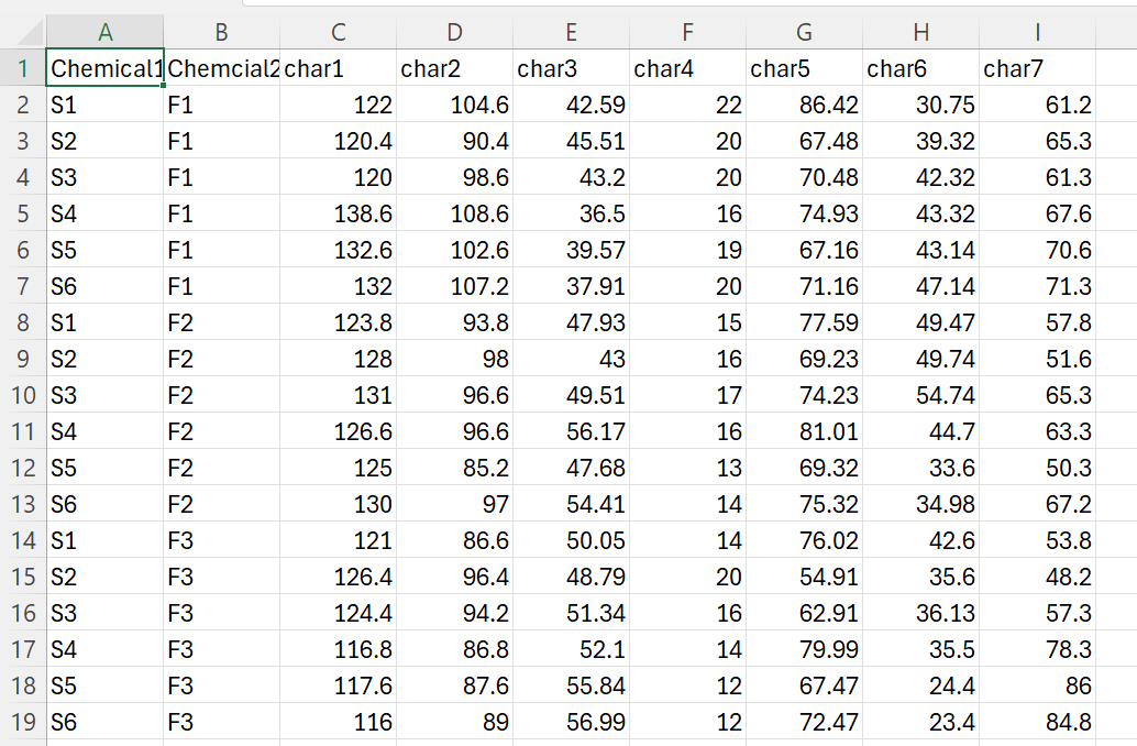
Because the full file runs to 90 rows, Figure 4 shows only the first replication (the 18 treatment combinations once each); in the complete dataset every combination appears on five rows.
8 The Analysis tab
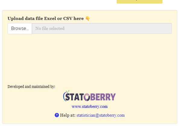
With your CSV ready, open the Analysis tab. The first step is to upload the file: click Browse… under Upload data file Excel or CSV here (Figure 5) and select your CSV. A blue Upload complete bar confirms the file has loaded.
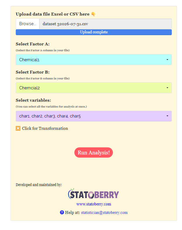
Once the file is in, RAISINS reads its column names and asks you to point it at the right columns (Figure 6):
- Select Factor A - the column holding the levels of the first factor (here,
Chemical1). - Select Factor B - the column holding the levels of the second factor (here,
Chemcial2). - Select variables - one or more response columns to analyse; you may select all of them at once (here
char1–char5), and RAISINS analyses each in turn. - Click for Transformation - an optional toggle to transform skewed responses before analysis (see below).
When the columns are chosen, click Run Analysis!. RAISINS fits the factorial model to every selected response and fills the results sub-tabs, Analysis Results, Basic Plots, Advanced Plots, Interpretation, Multivariate, FAQs and View Data.
You do not need to run the module once per response. Select all the response columns together and RAISINS produces a complete ANOVA, mean-comparison and effect-size table for each, plus a single MANOVA across all of them. This is why the results tables in the next section carry one column per trait.
8.1 Optional: transforming a response
The factorial ANOVA assumes the response is roughly normal with similar variability across treatments. When a trait is strongly skewed or its spread grows with its mean, tick Click for Transformation and choose a transformation before running the analysis. RAISINS offers the three standard choices and applies safe adjustments for awkward values:
| Transformation | Use it when | What RAISINS applies |
|---|---|---|
| Logarithmic | The spread grows in proportion to the mean (multiplicative data) | \(\log_{10}(x)\); if any value is \(\le 0\), it shifts first as \(\log_{10}(x - \min + 1)\) |
| Square-root | Counts, or data following a Poisson-like pattern | \(\sqrt{x}\); if any value is \(0\), it uses \(\sqrt{x + 0.5}\); negative values are not allowed |
| Arcsine | Proportions or percentages between 0 and 1 | \(\arcsin(\sqrt{x})\), with \(0\) and \(1\) nudged by \(1/(4n)\) so the transform stays finite |
A transformation is a temporary change of scale to make the test valid; it does not change your experiment. Report that a transformation was used, but discuss the means and recommendations in the original units. If no assumption is violated, leave the toggle off, an unnecessary transformation only makes the results harder to read.
9 Analysis results
The Analysis Results sub-tab is where the factorial ANOVA Results are loaded. A control panel at the top lets you set the multiple-comparison test (LSD by default, with Tukey’s HSD and Duncan’s DMRT as alternatives), the level of significance (\(\alpha\), 0.05 by default), the digits after decimal, and the font. A Quick Summary of the results and the dataset used is given below, and then presents four tables: the ANOVA summary, a Factor A table, a Factor B table, and the interaction (A × B) table. Every table carries one column per response (char1–char5).
Table 1: ANOVA summary - mean squares and significance
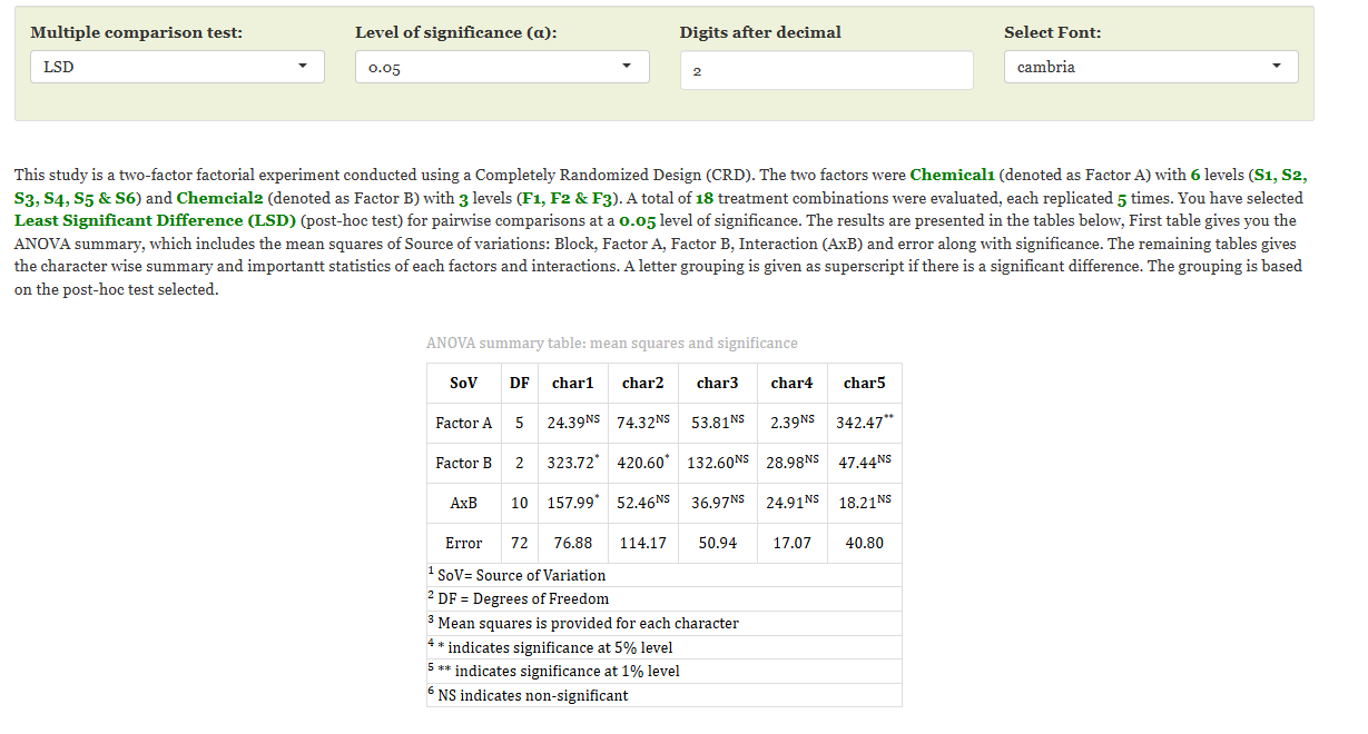
Each row is a source of variation, Factor A (5 df), Factor B (2 df), the interaction A × B (10 df) and Error (72 df), matching the degrees of freedom predicted in Section 2 for a \(6 \times 3 \times 5\) experiment. Each cell is that source’s mean square for the response, with a superscript flag: * for significance at 5%, ** at 1%, and NS for non-significant. Scanning the flags tells the whole story at a glance: char5 responds strongly to Factor A (\(342.47^{**}\)); char1 (\(323.72^{*}\)) and char2 (\(420.60^{*}\)) respond to Factor B; and char1 additionally carries a significant A × B interaction (\(157.99^{*}\)). By contrast char3 and char4 are NS for every source, unaffected by either chemical. Each significant cell is unpacked in the tables that follow.
How this table is built
RAISINS fits the linear model response ~ A + B + A:B for each trait and forms the analysis-of-variance table with Type II sums of squares. Each factor’s mean square is its sum of squares divided by its degrees of freedom, and the F-test divides it by the error mean square; the p-value behind each F decides the * / ** / NS flag against the chosen \(\alpha\). This is the many-level generalisation of the \(2 \times 2\) contrasts in Section 4.
Table 2: Factor A - means and comparison statistics
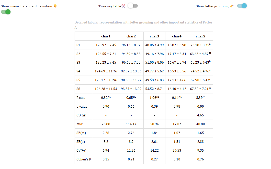
This table averages over Factor B to show the main effect of Factor A (the six levels S1–S6). The one response Factor A affects is char5: \(F = 8.39^{**}\) (\(p = 0.00\)), with a critical difference CD (A) of 4.65 and a large Cohen’s F of 0.76. The letter groupings on char5 rank the chemicals: S4 (\(74.52 \pm 4.76\)) and S1 (\(73.18 \pm 8.35\)) share letter a as the highest, while S5 (\(62.90 \pm 6.47\), letter c) is the lowest. For char1–char4 the F-statistics are non-significant, so their CD (A) rows read “–”, RAISINS withholds the post-hoc test in that case. The lower rows report the pooled MSE, the standard error of a mean SE(m) and of a difference SE(d), the coefficient of variation CV(%), and the Cohen’s F effect size.
Table 3: Factor B - means and comparison statistics
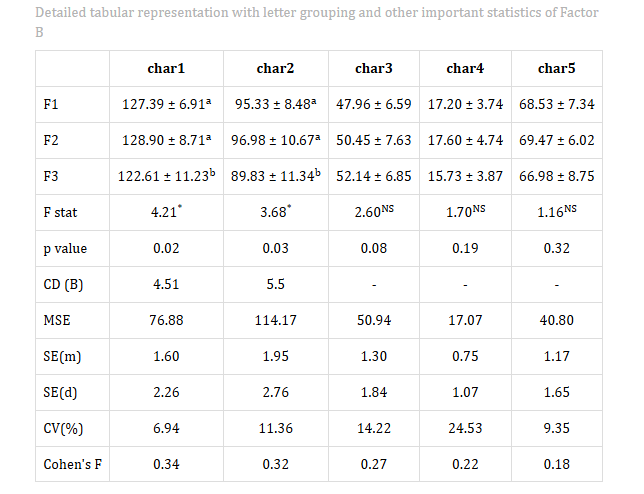
The Factor B table has the same layout, now averaging over Factor A to show the main effect of Factor B across its three levels (F1, F2, F3). Factor B is significant for two responses. For char1, \(F = 4.21^{*}\) (\(p = 0.02\), CD (B) \(= 4.51\)): F1 (\(127.39 \pm 6.91\)) and F2 (\(128.90 \pm 8.71\)) share letter a, while F3 (\(122.61 \pm 11.23\), letter b) is significantly lower. For char2 the pattern repeats: \(F = 3.68^{*}\) (\(p = 0.03\), CD (B) \(= 5.5\)), with F1 and F2 on par (letter a) and F3 (\(89.83 \pm 11.34\), letter b) lowest. So the third level of Chemcial2 depresses both char1 and char2; for char3–char5 no level of Factor B stands out.
Table 4: Interaction A × B - cell means and comparison statistics
| Combination | char1 | char2 | char3 | char4 | char5 |
|---|---|---|---|---|---|
| S1×F1 | 123.52 ± 5.72abc | 97.04 ± 6.30 | 46.94 ± 4.94 | 16.00 ± 4.74 | 76.39 ± 8.16 |
| S1×F2 | 130.24 ± 10.06a | 100.24 ± 10.06 | 46.63 ± 5.96 | 19.20 ± 3.83 | 70.54 ± 6.80 |
| S1×F3 | 127.00 ± 5.66ab | 91.10 ± 9.31 | 50.60 ± 3.86 | 15.40 ± 2.79 | 72.63 ± 10.45 |
| S2×F1 | 125.68 ± 8.00abc | 92.72 ± 8.70 | 48.21 ± 6.84 | 15.80 ± 4.27 | 63.64 ± 6.21 |
| S2×F2 | 125.48 ± 9.49abc | 95.52 ± 9.55 | 45.93 ± 10.75 | 20.80 ± 6.87 | 65.60 ± 3.60 |
| S2×F3 | 128.48 ± 4.58a | 94.92 ± 8.56 | 53.33 ± 4.86 | 15.80 ± 3.70 | 61.66 ± 4.67 |
| S3×F1 | 124.20 ± 6.45abc | 95.72 ± 8.63 | 48.10 ± 9.42 | 14.80 ± 4.44 | 67.84 ± 6.10 |
| S3×F2 | 128.92 ± 9.50a | 98.36 ± 8.54 | 49.27 ± 7.57 | 19.40 ± 3.36 | 71.20 ± 2.19 |
| S3×F3 | 131.56 ± 5.27a | 95.88 ± 6.84 | 55.61 ± 6.37 | 15.80 ± 1.79 | 65.66 ± 2.68 |
| S4×F1 | 130.64 ± 7.23a | 95.32 ± 12.21 | 48.15 ± 6.85 | 17.80 ± 2.05 | 74.14 ± 3.27 |
| S4×F2 | 127.56 ± 10.32ab | 98.36 ± 11.96 | 52.66 ± 4.67 | 15.80 ± 2.68 | 74.99 ± 7.01 |
| S4×F3 | 115.88 ± 13.19c | 84.04 ± 13.80 | 48.49 ± 6.11 | 16.00 ± 5.48 | 74.44 ± 4.37 |
| S5×F1 | 129.76 ± 8.78a | 94.24 ± 9.39 | 47.47 ± 6.22 | 19.40 ± 2.97 | 61.80 ± 4.24 |
| S5×F2 | 128.68 ± 7.96a | 91.64 ± 11.55 | 52.02 ± 7.08 | 16.20 ± 5.50 | 65.26 ± 4.91 |
| S5×F3 | 116.92 ± 12.38bc | 86.16 ± 13.45 | 49.24 ± 7.83 | 15.80 ± 5.12 | 61.65 ± 9.69 |
| S6×F1 | 130.52 ± 3.24a | 96.96 ± 8.78 | 48.87 ± 8.13 | 19.40 ± 1.95 | 67.40 ± 3.82 |
| S6×F2 | 132.52 ± 7.91a | 97.76 ± 15.04 | 56.15 ± 6.81 | 14.20 ± 3.35 | 69.26 ± 6.41 |
| S6×F3 | 115.80 ± 13.55c | 86.88 ± 14.32 | 55.55 ± 10.60 | 15.60 ± 5.13 | 65.85 ± 10.92 |
| F stat | 2.05* | 0.46NS | 0.73NS | 1.46NS | 0.45NS |
| p value | 0.04 | 0.91 | 0.70 | 0.17 | 0.92 |
| CD (A×B) | 11.05 | – | – | – | – |
| MSE | 76.88 | 114.17 | 50.94 | 17.07 | 40.80 |
| SE(m) | 3.92 | 4.78 | 3.19 | 1.85 | 2.86 |
| SE(d) | 5.55 | 6.76 | 4.51 | 2.61 | 4.04 |
| CV(%) | 6.94 | 11.36 | 14.22 | 24.53 | 9.35 |
| Cohen’s F | 0.53 | 0.25 | 0.32 | 0.45 | 0.25 |
Cell values are mean ± SD. Where the interaction is significant (char1), superscript letters give the post-hoc grouping - combinations sharing a letter are not significantly different. * marks significance at 5%, ** at 1%, NS non-significant. MSE, SE and CV(%) are common to each response.
This is the Interaction effect table. Its rows are the eighteen treatment combinations, each level of Chemical1 crossed with each level of Chemcial2 (S1×F1, S1×F2, S1×F3, …, S6×F3), shown as mean ± SD. When the interaction is significant for a response, a letter grouping appears as a superscript: combinations sharing a letter are not significantly different. The one response with a significant interaction is char1: \(F = 2.05^{*}\) (\(p = 0.04\)) with a critical difference of 11.05 and a Cohen’s F of 0.53.
Reading every row of the factor tables
- Mean ± SD - the treatment (or cell) mean and its standard deviation; a transformed mean, if a transformation was applied, is shown in parentheses.
- F stat / p value - the F-test for that source and its probability; the superscript (
*,**,NS) marks significance at the chosen \(\alpha\). - CD - the critical difference (from the selected post-hoc test); two means differing by more than the CD are significantly different. Shown as “–” when the source is non-significant or the design is unbalanced.
- MSE - the pooled error mean square, common to all comparisons of that response.
- SE(m) / SE(d) - standard error of a single mean and of a difference between two means.
- CV(%) - coefficient of variation, the error SD as a percentage of the grand mean; it gauges experimental precision and is common to the whole experiment.
- Cohen’s F - a standardised effect size for the source (roughly: below 0.10 very small, 0.25 small, 0.40 medium, above 0.40 large).
A significant effect tells you the pattern is unlikely to be chance; it does not, by itself, tell you the difference is large enough to matter. Read the Cohen’s F effect size alongside the p-value, For example, in the char5, Factor A effect is not only significant but also have a large (Cohen’s F 0.76).
10 Visualising the results
RAISINS groups its graphics into two sub-tabs, Basic Plots and Advanced Plots, and every plot can be redrawn for any factor and any response, then exported as PNG, JPEG, TIFF, PDF or SVG.
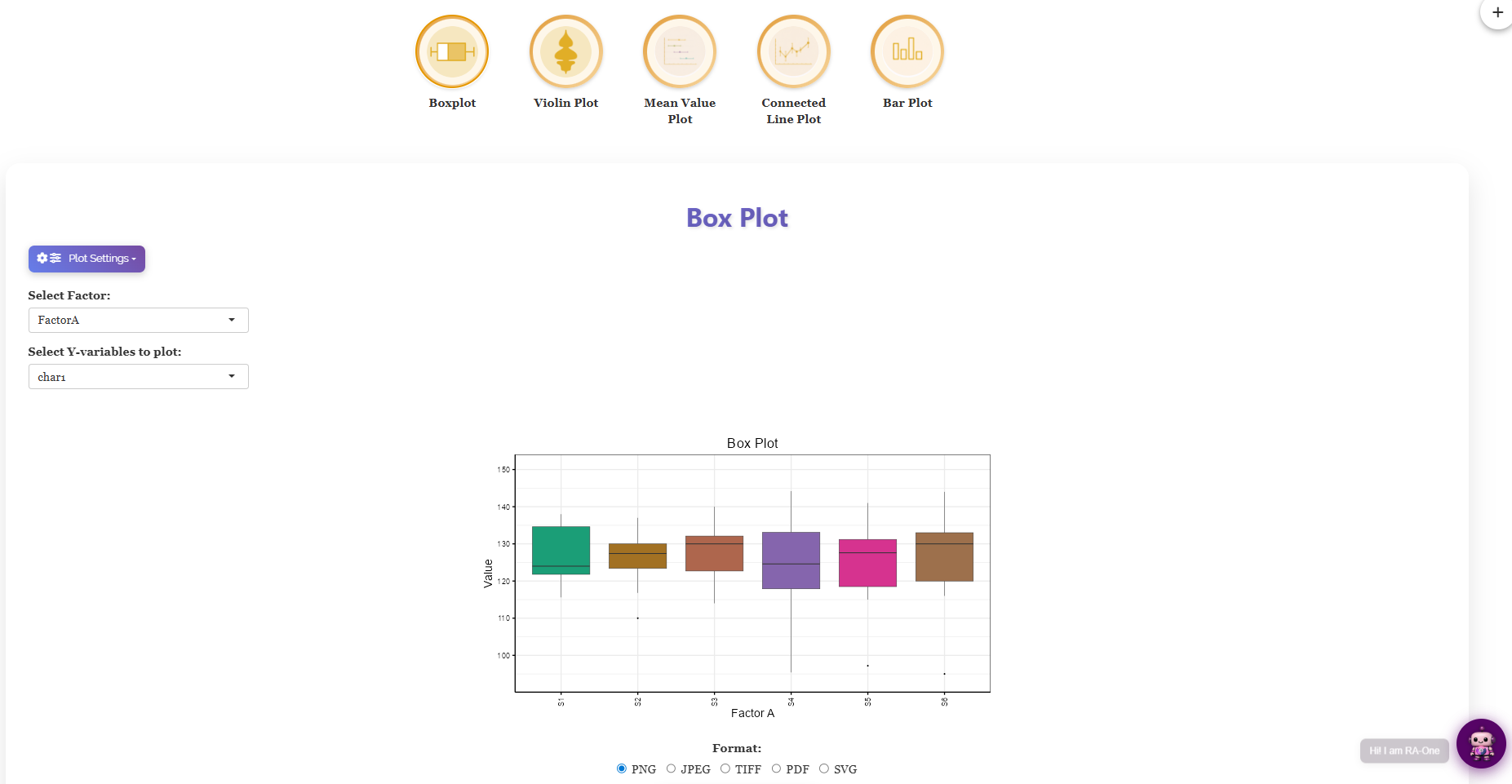
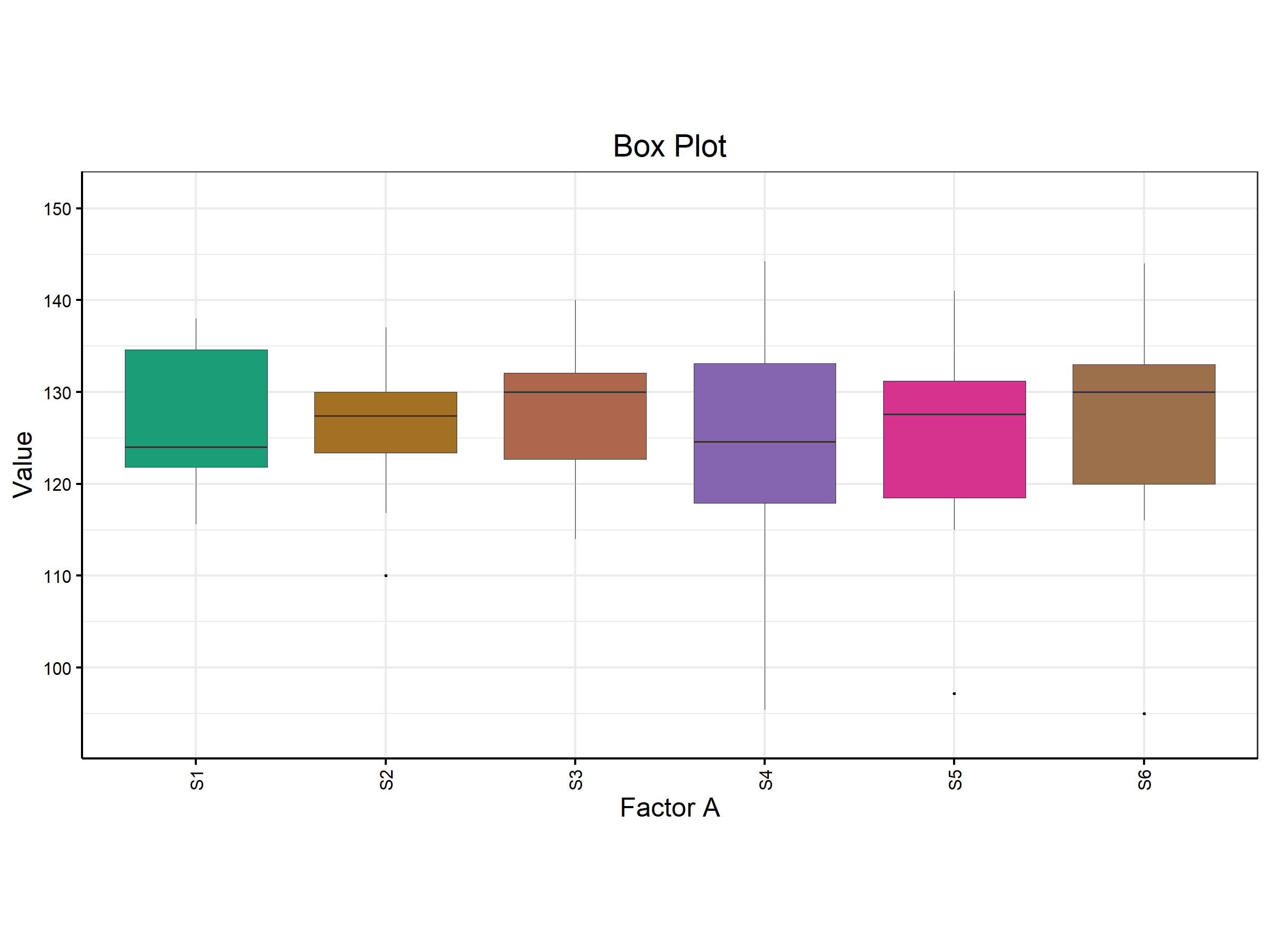
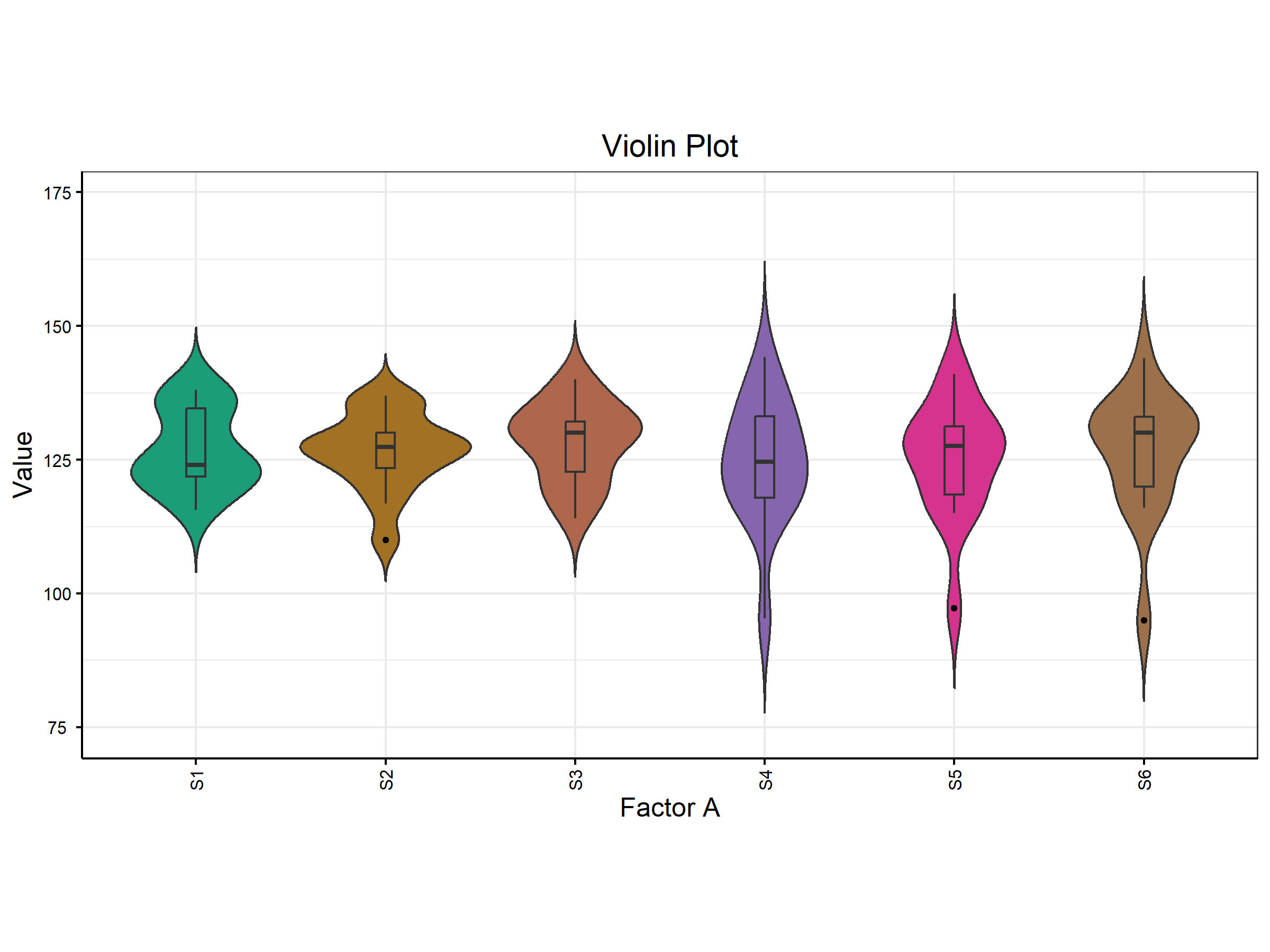
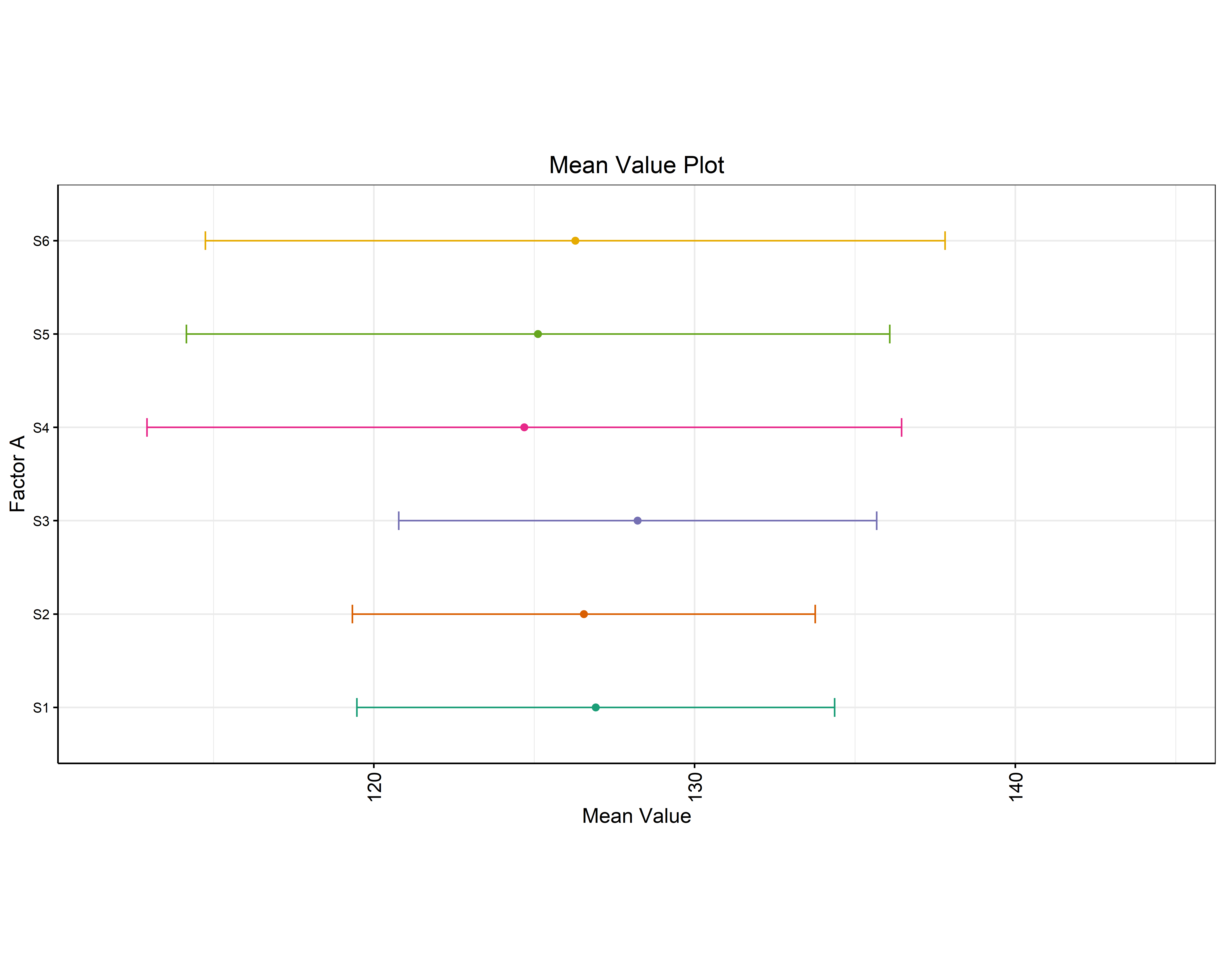
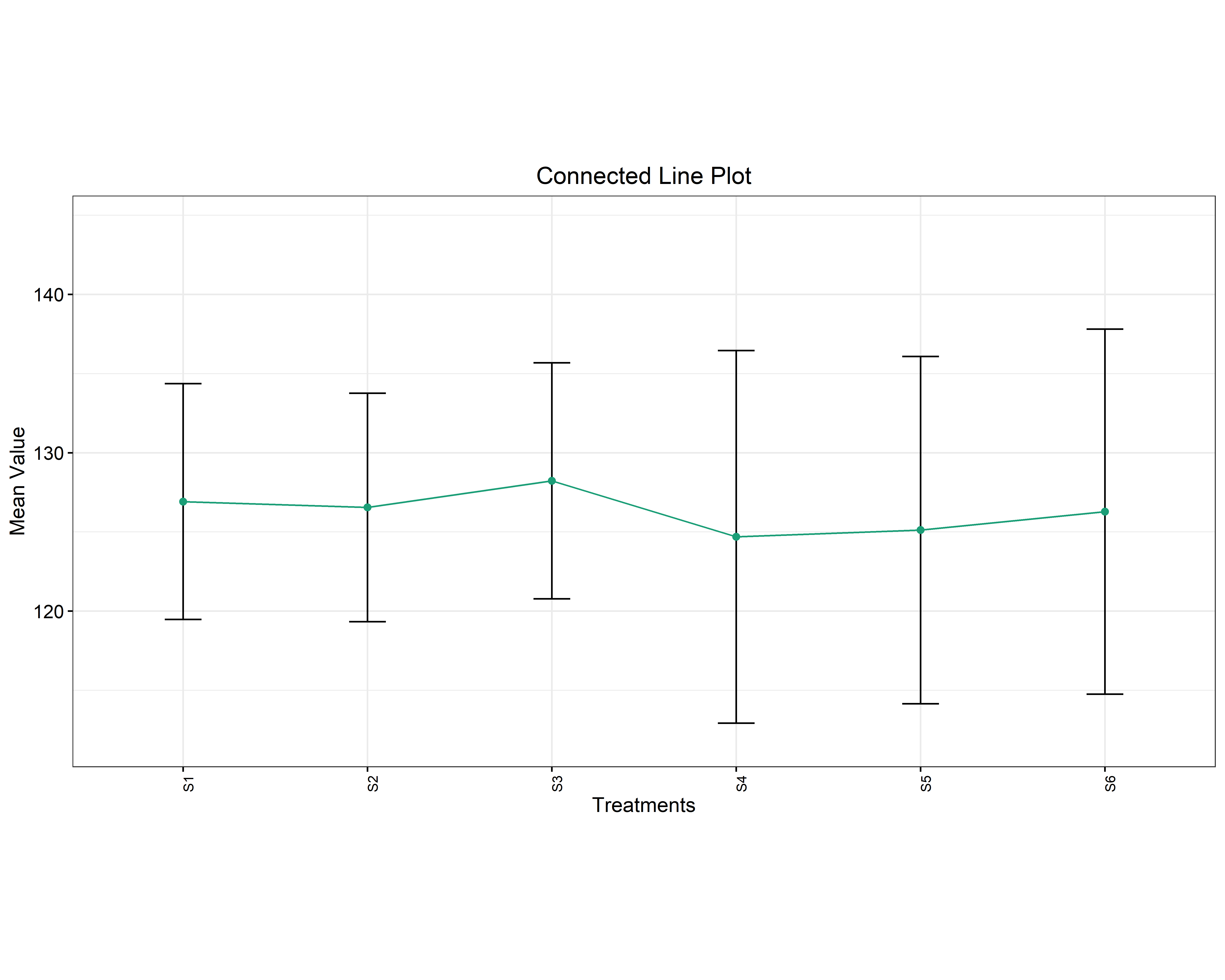
The Basic Plots tab (Figure 10) offers plots like, Boxplot, Violin Plot, Mean Value Plot, Connected Line Plot and Bar Plot. Choose the factor to place on the x-axis (Chemical1, Chemcial2, or the interaction) and the response to plot. Figure 11 draws the same char1-by-Chemical1 comparison four ways, the six levels S1–S6 overlap heavily, the visual echo of the non-significant Factor A effect on char1 from Figure 8.
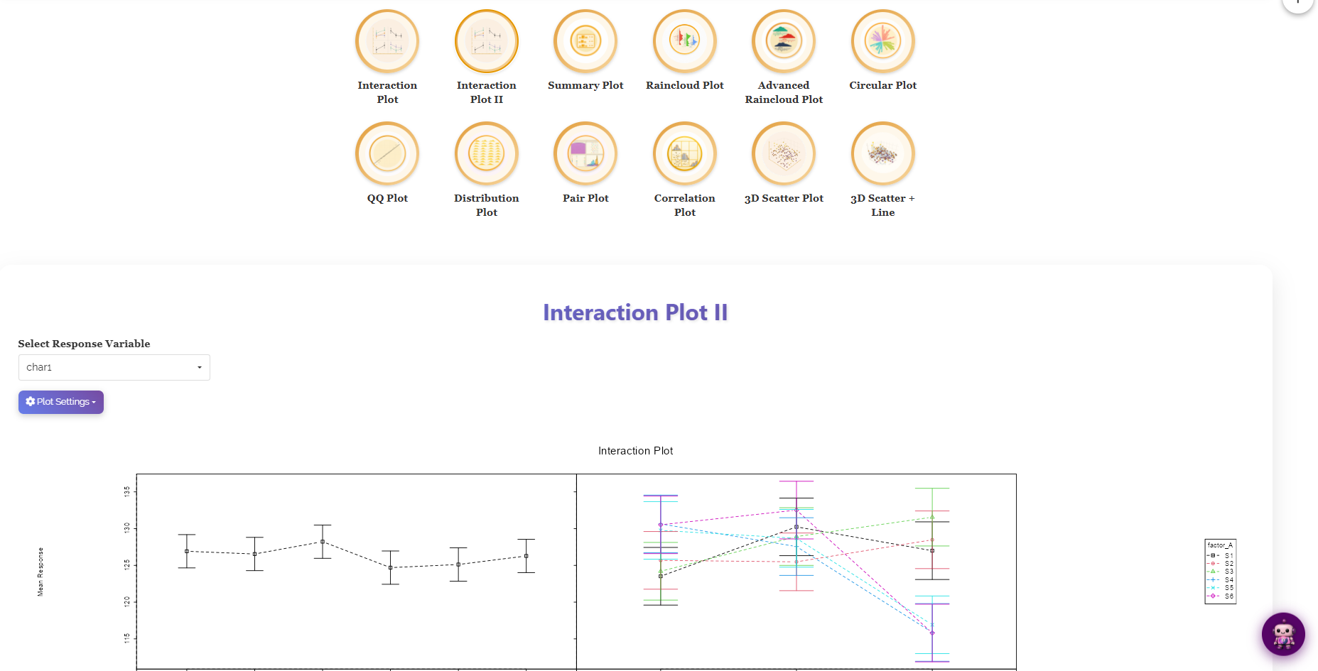
The Advanced Plots tab (Figure 12) adds the specialised graphics: two Interaction Plots, a Summary Plot, Raincloud and Advanced Raincloud, a Circular Plot, a QQ Plot, a Distribution Plot, a Pair Plot, a Correlation Plot, and 3-D Scatter views.
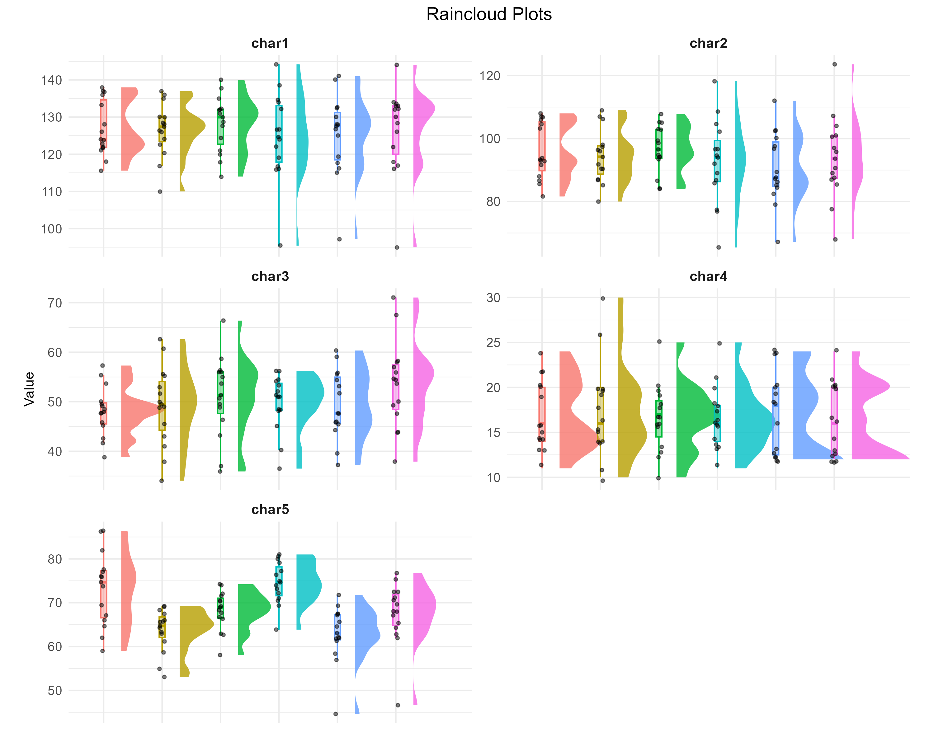
Two Advanced plots earn special attention in a factorial study:
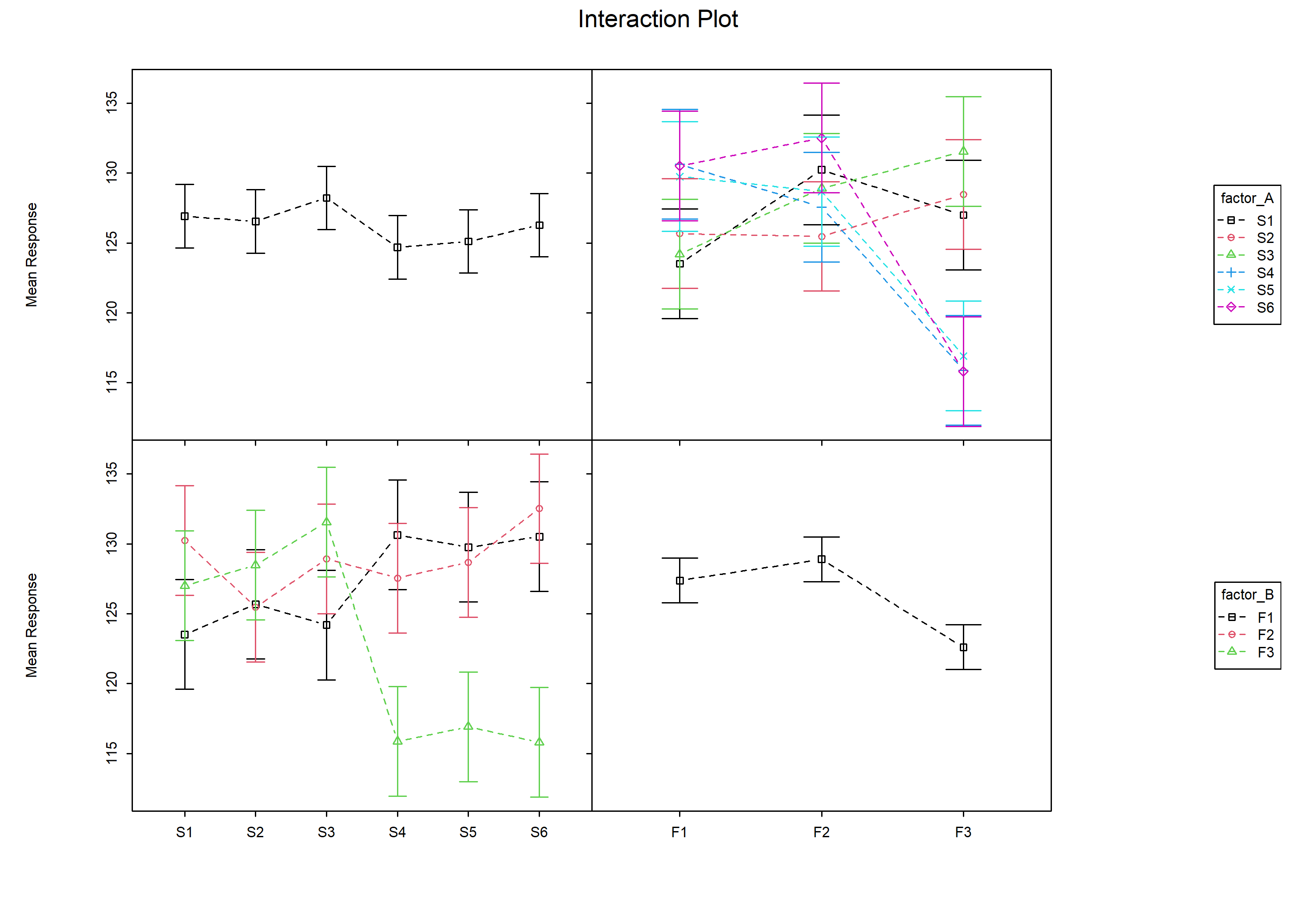
- The Interaction Plot draws the mean response for each Chemcial2 level as a line across Chemical1 (or vice versa). Parallel lines signal no interaction; lines that cross or fan apart signal one, this is the visual form of the interaction contrast from Section 4, and the natural companion to the char1 finding in Table 4.
- The QQ Plot checks the normality assumption behind the ANOVA: it plots the model residuals against the values expected under a normal distribution. Points hugging the straight line support normality; a strong curve or S-shape suggests a transformation (Section 8) may be needed.
11 Looking at all traits together: MANOVA and PCA index
The Analysis Results tab tests each trait one at a time. Sometimes you want to know whether the treatments differ when all the traits are considered together, or to combine the traits into a single selection index. The Multivariate tab (Figure 14) provides both tools: a MANOVA and a PCA-based index score. RAISINS lists the response variables entering the multivariate study and offers two buttons, Click here for MANOVA and Click here for PCA Index.
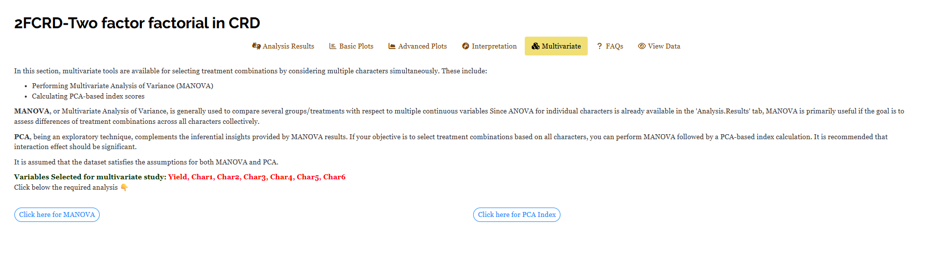
11.1 MANOVA across all responses
MANOVA (Multivariate Analysis of Variance) asks whether the treatment combinations differ when the five traits are treated as one bundle. RAISINS fits the two-way model with interaction and reports Pillai’s trace, the most robust multivariate test statistic, converted to an F-value (Figure 15). Here Factor A is significant across the combined traits (Pillai \(= 0.54\), \(F = 1.75\), \(p = 0.02\)), echoing its strong univariate effect on char5, while Factor B (Pillai \(= 0.21\), \(F = 1.60\), \(p = 0.11\)) and the interaction A × B (Pillai \(= 0.64\), \(F = 1.05\), \(p = 0.39\)) are non-significant when all traits are pooled. The partial \(\eta^2\) column (0.11, 0.10, 0.13) reports effect sizes; a moderate \(\eta^2\) can accompany a non-significant test, so the p-values remain the deciding evidence.
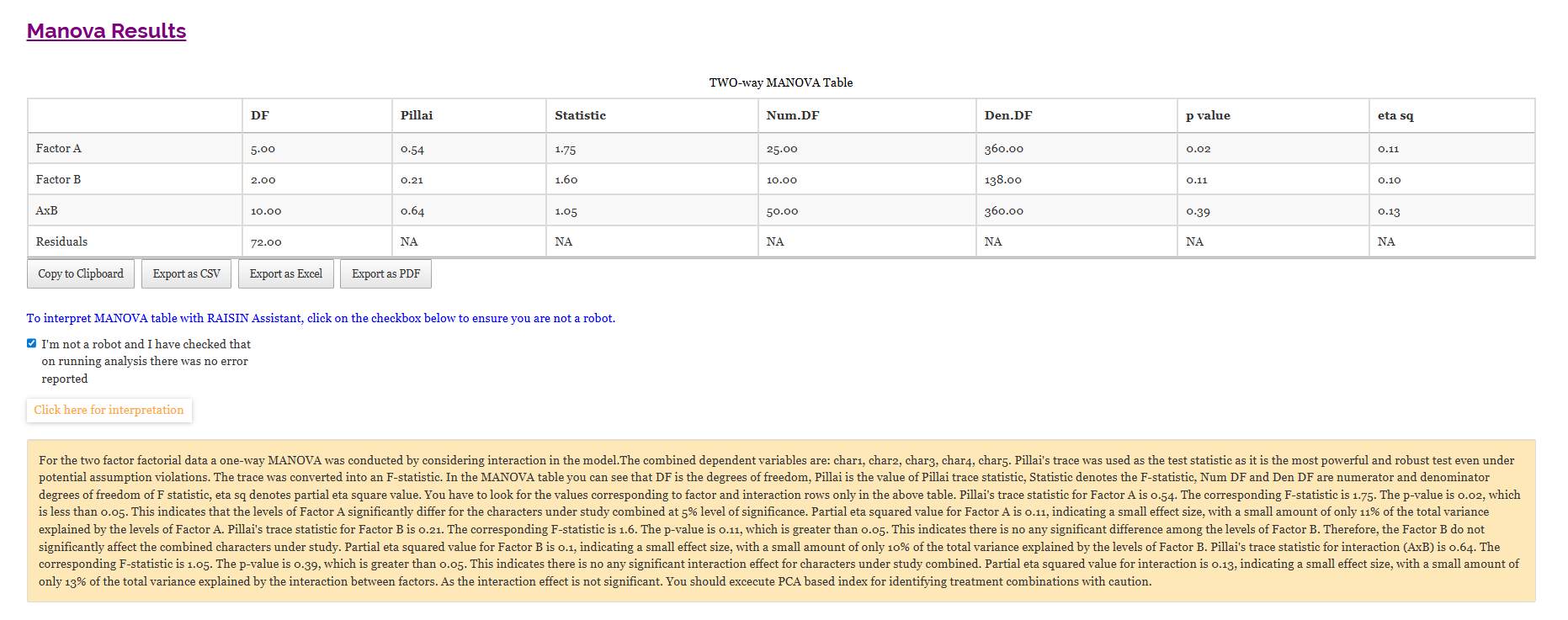
11.2 PCA-based index score
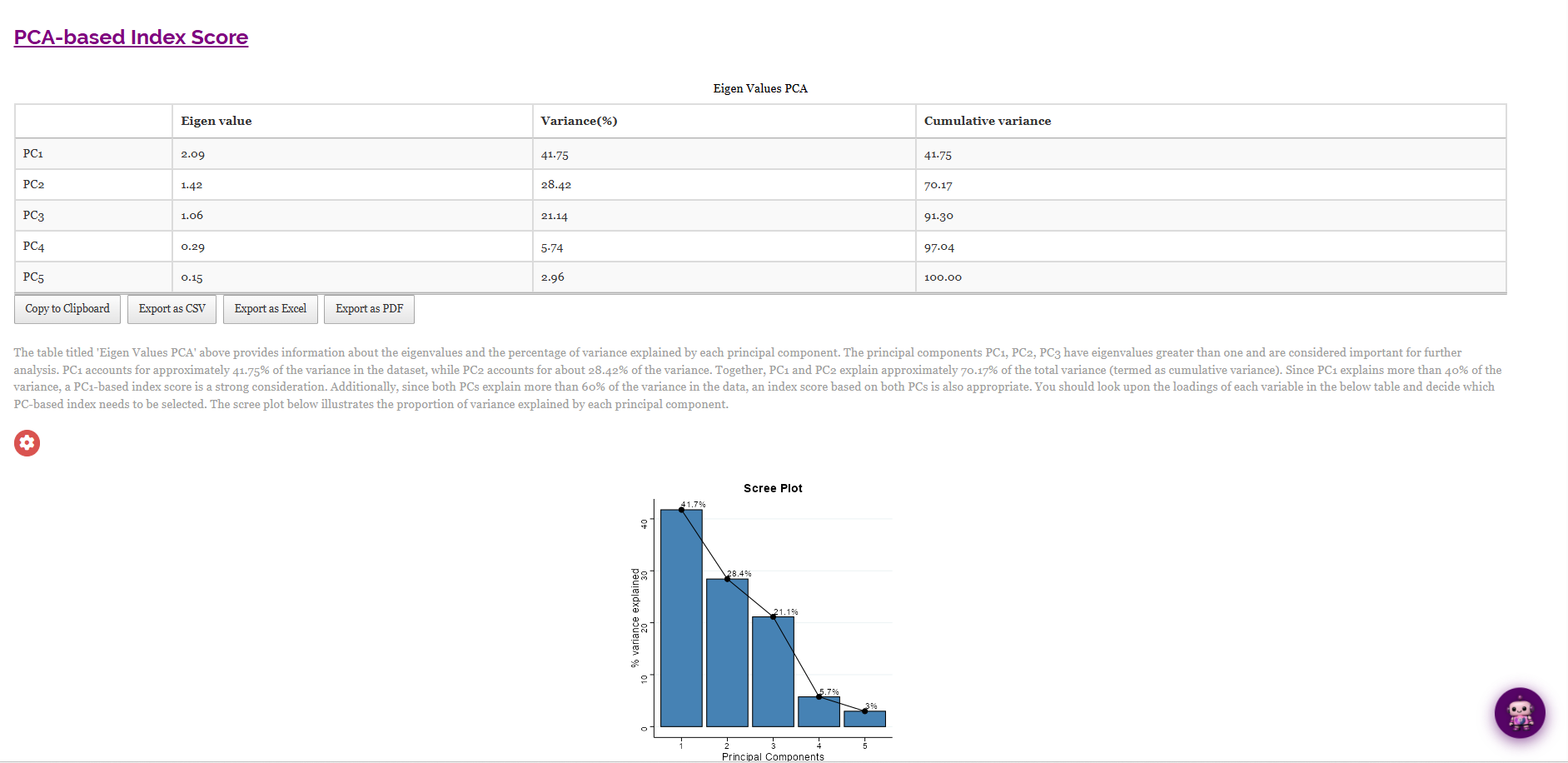
When you want to rank treatment combinations on all traits at once, the PCA-based index condenses the correlated traits into a few independent components and builds a score from them. The eigenvalue table (Figure 16) shows how much variance each component captures: PC1 explains 41.75% and PC2 28.42%, together 70.17% of the total variation, more than enough for a meaningful two-component index. The accompanying scree plot shows the same information graphically, the variance explained falling away after the first three components. To decide which index to use, read the loadings of each trait on the components (Figure 17): char3 loads positively on PC1 while char1, char2, char4 and char5 load negatively, so a PC1 score separates char3 from the rest. The biplot places each treatment combination in the direction of the traits it scores highly on.
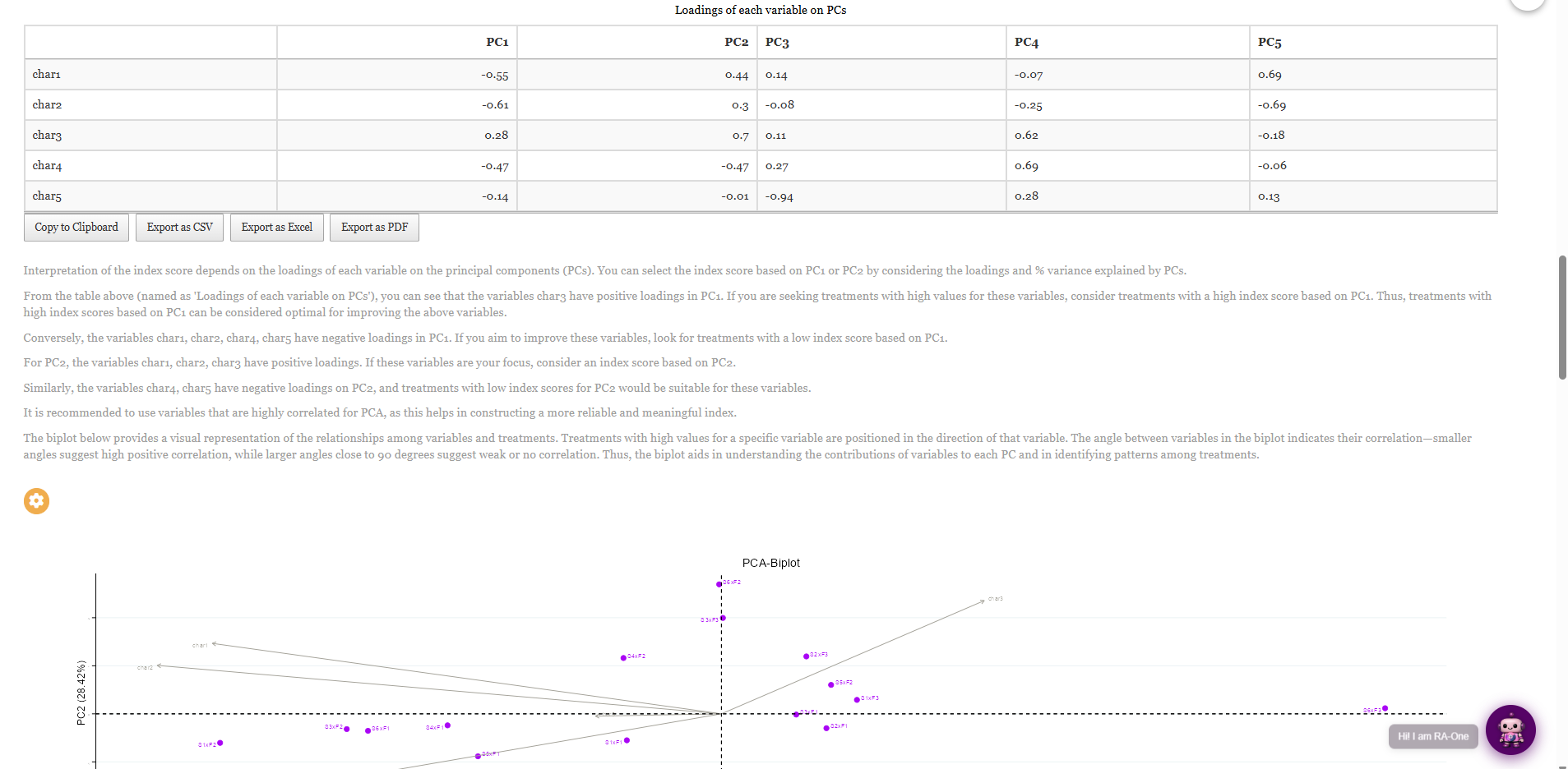
MANOVA is inferential, does any treatment differ across the traits collectively? PCA is exploratory, how can the traits be combined into an index to rank treatments? They complement each other. Here the interaction is not significant in the MANOVA, and RAISINS itself advises running the PCA index with caution when the interaction is non-significant, since that is when ranking a single “best combination” is least clear-cut.
12 Interpretation
RAISINS provides a clear, plain-language interpretation of your results so you can understand the findings without decoding the tables yourself. Open the Interpretation sub-tab, confirm you are not a robot, and click Click here for interpretation (Figure 18). RAISINS restates the design, then reads every response for you: which main effects and interactions were significant, what the post-hoc letter groupings mean, and how large the effects are. For the working dataset it reports the Factor A effect on char5 (S4 highest at \(74.52 \pm 4.76\), S5 lowest at \(62.90 \pm 6.47\)), the Factor B effects on char1 and char2 (F3 the lowest level in both), and the significant interaction on char1 (\(p = 0.04\)), with S6×F2 highest (\(132.52 \pm 7.91\)) and S6×F3 lowest (\(115.80 \pm 13.55\)), spelling out which combinations are statistically on par. The text is written to be pasted almost directly into a results section.

The interpretation is generated from the same computation as the tables, so use it as a guide, not a substitute. Read it with Figure 7 and Table 4 open beside it, the numbers in the prose should match the numbers in the tables exactly, which is your quickest check that you selected the right columns.
13 Chat with your data using RA-One
RA-One is the built-in conversational assistant for the two-factor factorial module, available from the RA-One tab. You ask questions in plain language and it answers using your own analysis rather than generic statistical advice. Every result it discusses is drawn from what the module actually computed, it never invents numbers, and if a value isn’t available it says so instead of guessing. All answers are in plain English, with no code or software commands.
Once your results are loaded, RA-One greets you and offers quick-start prompts (Figure 19): Guide me through my results for a step-by-step walkthrough, Interpret results to summarise the significance of each character, Best treatment to ask which combination performs best across all traits, and Report results to help draft the write-up. You can also type your own question, for example “is the interaction significant for any trait?” or “which Chemcial2 level gives the highest char2?”.

The same chat window can also prepare your data. It can build a correctly formatted design template (Section 3.2) for you to fill in, or fetch the model dataset so you can try the module straight away, so you never need to leave the tab to get a file ready.
Within a single conversation, RA-One can interpret your results, build a data template, fetch the model dataset, and guide you through the tables, so most of a routine two-factor factorial session can be conducted without ever leaving the chat window.
14 FAQs
The module includes a dedicated FAQs sub-tab to clear up common doubts and guide you through the features, with detailed answers and practical tips. Typical questions include “my design is unbalanced, why is the critical difference shown as a dash?” and “the interaction is significant but neither main effect is, how do I report that?”, both of which arise naturally with factorial data.
15 View data
View Data is the primary diagnostic tool for ensuring data integrity before analysis. When you upload your dataset, RAISINS runs an automated Health Check to validate the file: it confirms that the two factor columns are present and read as categorical labels, that the response columns are numeric, and that there are no stray blanks or misaligned rows. For a factorial design it also checks that every factorA × factorB combination is present and reports whether the replication is balanced, the condition under which the standard errors and critical differences are exact. Fix any flagged issue here before trusting the results.
16 Wrapping up
A two-factor factorial CRD exists to answer one honest question: do two factors act independently, or does the effect of one depend on the other? Everything in this module, the ANOVA summary, the Factor A and Factor B tables, the interaction table, the plots, the MANOVA and the interpretation, exists to answer that question fairly, and to tell you the cell means to act on when the answer is “they interact.”
This module fits the case where your experimental units are homogeneous, so the treatments can be assigned completely at random. If your units are not uniform and you had to group them to control a gradient, use the factorial RBD module instead; if you are studying a single factor, use the one-way CRD module. And if you get stuck at any point, RA-One is available 24 × 7, or write to us at [email protected].
