Canonical Correlation Analysis
Canonical correlation analysis finds the strongest linear relationship between two whole sets of variables at once. This tutorial explains what a canonical variate and a canonical correlation are, how RAISINS decides which functions are worth interpreting, how to read the loading tables, and how to run the whole analysis code-free… Read more …
Canonical Correlation Analysis (CCA) is a multivariate statistical technique for studying the relationship between two whole sets of variables at once, rather than between a single pair. It finds the linear combination of each set that correlates most strongly with the other, then repeats the search for additional, independent dimensions of relationship.
This tutorial introduces the basic concepts of canonical correlation analysis, including canonical variates, canonical correlations, Wilks’ Lambda, and structure and cross-loadings. It then provides a step-by-step guide to performing canonical correlation analysis in the RAISINS platform. You will learn how to prepare your data, select the X-set and Y-set variables, interpret the analysis results, review the plots, and use the built-in RA-One AI assistant to better understand your results. No programming knowledge is required.
1 What is Canonical Correlation Analysis?
Suppose you ran a pot-culture trial on 55 plants. For each plant, you recorded four growing conditions - temperature, sunlight hours, water supplied, and fertilization - and four development outcomes - height, leaf count, biomass, and flower count. You want to know whether growing conditions, taken together, relate to plant development, taken together.
An ordinary correlation only ever compares two single variables at a time, so you would need to compute and interpret sixteen separate correlations (four growing-condition variables against four development variables) and would still learn nothing about how the two sets act as a whole. Canonical correlation analysis (CCA) answers the whole-set question directly. It studies the relationship between an X-set of variables (here, growing conditions) and a Y-set of variables (here, development outcomes).
CCA does this by constructing two new variables: a canonical variate U, a weighted combination of the X-set variables, and a canonical variate V, a weighted combination of the Y-set variables. The weights are chosen so that U and V correlate with each other as strongly as possible. This single number, the correlation between U and V, is the canonical correlation.
One pair of canonical variates rarely tells the whole story. CCA extracts additional pairs, each capturing an independent, uncorrelated dimension of relationship the first pair missed. The number of pairs is always min(p, q), where p and q are the number of variables in the X-set and Y-set. With 4 variables in each set here, CCA extracts 4 canonical functions.
Canonical correlation analysis finds the linear combination of one set of variables and the linear combination of a second set of variables that correlate with each other as strongly as possible, then repeats the search for additional, independent dimensions of relationship.
1.1 Canonical variates, loadings, and cross-loadings
Each canonical function produces several related quantities, and it is easy to confuse them. RAISINS reports all of them separately.
- A raw canonical coefficient is a weight in the linear combination that defines a canonical variate, comparable to a regression coefficient. It is in standardized units and is rarely interpreted directly.
- A structure loading is the ordinary Pearson correlation between one original variable and the canonical variate built from its own set. It is easier to interpret than a raw coefficient: a loading close to +1 or -1 means that variable strongly defines the canonical variate; a loading close to 0 means it contributes little.
- A cross-loading is the correlation between one original variable and the canonical variate of the other set. It shows how strongly a variable relates to the pattern found on the opposite side.
\[U = a_1X_1 + a_2X_2 + \cdots + a_pX_p \qquad V = b_1Y_1 + b_2Y_2 + \cdots + b_qY_q\]
\[\rho = \operatorname{cor}(U, V)\]
Canonical correlation analysis is not the same as running a regression of one set on the other, and it does not identify which individual X variable predicts which individual Y variable. It finds the single best-correlated pair of composite variables, one built entirely from the X-set and one built entirely from the Y-set. To see which original variables actually drive that relationship, read the loadings, not the raw coefficients.
CCA also describes association, not causation. A strong canonical correlation between growing conditions and plant development is evidence of a relationship in this dataset; it does not, by itself, prove that changing one set of variables would change the other.
2 Which Canonical Functions Matter?
Not every canonical function extracted is worth interpreting. RAISINS uses two criteria together, matching the rule already shown in the app’s own results table:
- Statistical significance - tested with Wilks’ Lambda, a sequential test that asks whether canonical function k through the last one jointly explain more shared variance than chance. RAISINS reports the test statistic, its F-approximation, degrees of freedom, and a p-value for each function.
- Practical importance - the function’s r-squared (the canonical correlation squared), which is the proportion of variance the two composite variables share.
A canonical function is flagged Retained for interpretation only when its Wilks’ Lambda p-value is below the selected significance level and its r-squared is at least 0.10. A function can pass the significance test and still be skipped if it explains too little shared variance to matter in practice; large sample sizes routinely make tiny effects “significant”.
A Level of significance (α) dropdown lets you choose 0.05 (the default) or 0.01 for the Wilks’ Lambda test. Changing it re-evaluates which functions are marked “Retained” using the new threshold, without needing to re-run the analysis. A stricter α = 0.01 requires stronger evidence before a function counts as statistically significant, so a function with a p-value between 0.01 and 0.05 would move from “Retained” to “not retained” when you switch levels - none of the four functions in the worked example below are that close to the boundary, but it matters on datasets with weaker effects.
3 Getting to the Module
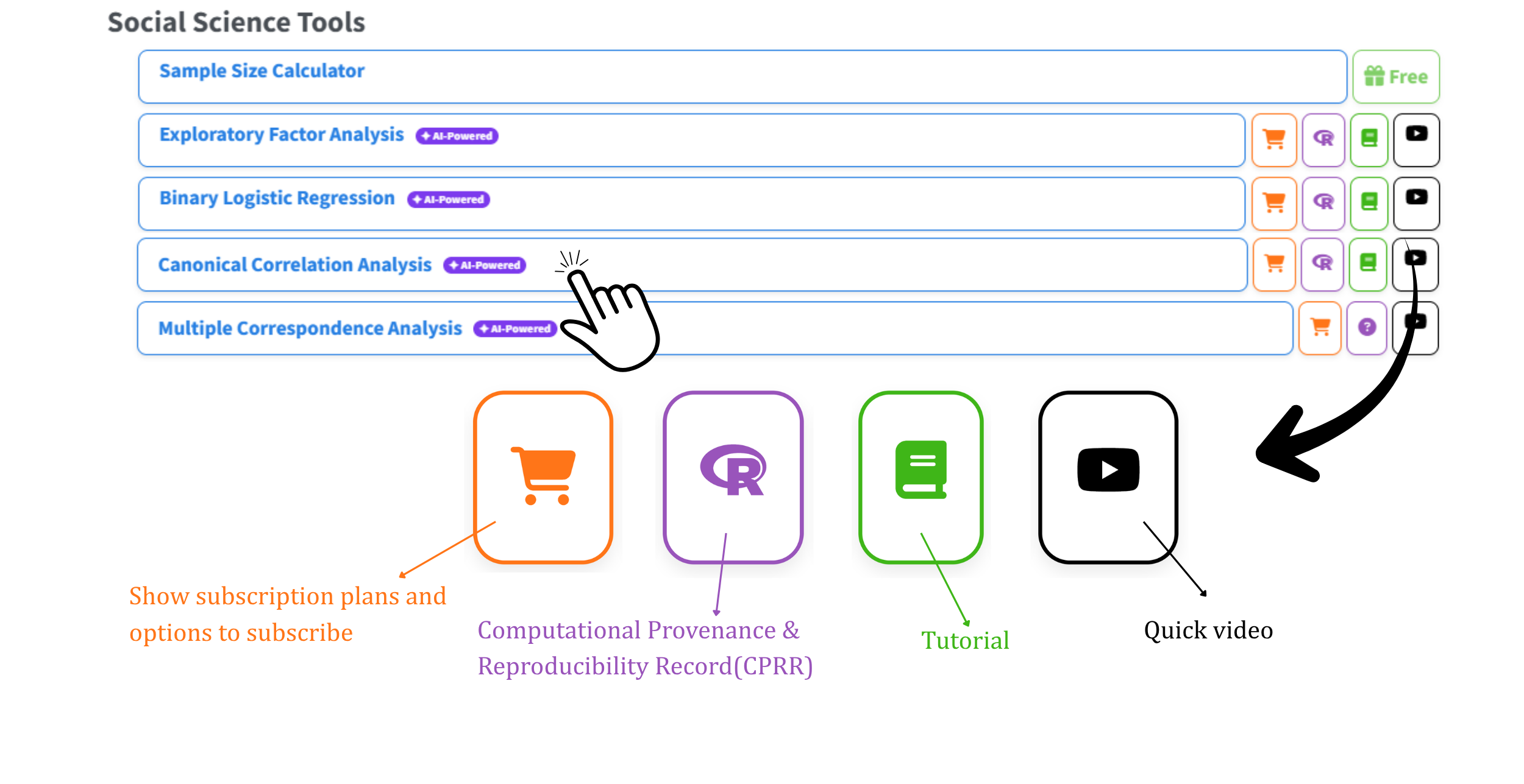
Open the RAISINS home page at www.raisins.live and go to the Social Science Tools section. Select the Canonical Correlation Analysis module (Figure 1).
No programming knowledge is required. You upload your data, select the X-set and Y-set variables, and RAISINS performs the complete analysis and produces publication-ready output.
3.1 Computational Provenance & Reproducibility Record
CPRR (Computational Provenance & Reproducibility Record) provides a transparent and comprehensive record. Click on the icon shown in Figure 1 to access CPRR and know about the computational workflow performed during the analysis. The record for this module states the R version and the exact version of every package used, names the specific function behind each reported result. CPRR lists every default parameter and decision rule applied by the module and provides fully runnable R code that reproduces each analytical step. Users can execute the code in R to independently reproduce and verify the results. It carries its own DOI.
To cite the platform itself in a paper, thesis, or report, use the RAISINS citation, available in APA, Harvard, and BibTeX formats at www.raisins.live/citation.html. That is the primary reference, and for most manuscripts it is all you need.
The CPRR for the canonical correlation analysis module is at www.raisins.live/module_record/cca.html.
Cite the RAISINS paper as your primary reference for the platform. Add the CPRR as supporting documentation when a journal asks for details of the computing environment, or when you want your methods section to be precise about versions and functions rather than saying “analysis was carried out using an online tool.” The CPRR supports the citation and ensures computational reproducibility.
4 Preview Mode and Quick Tour
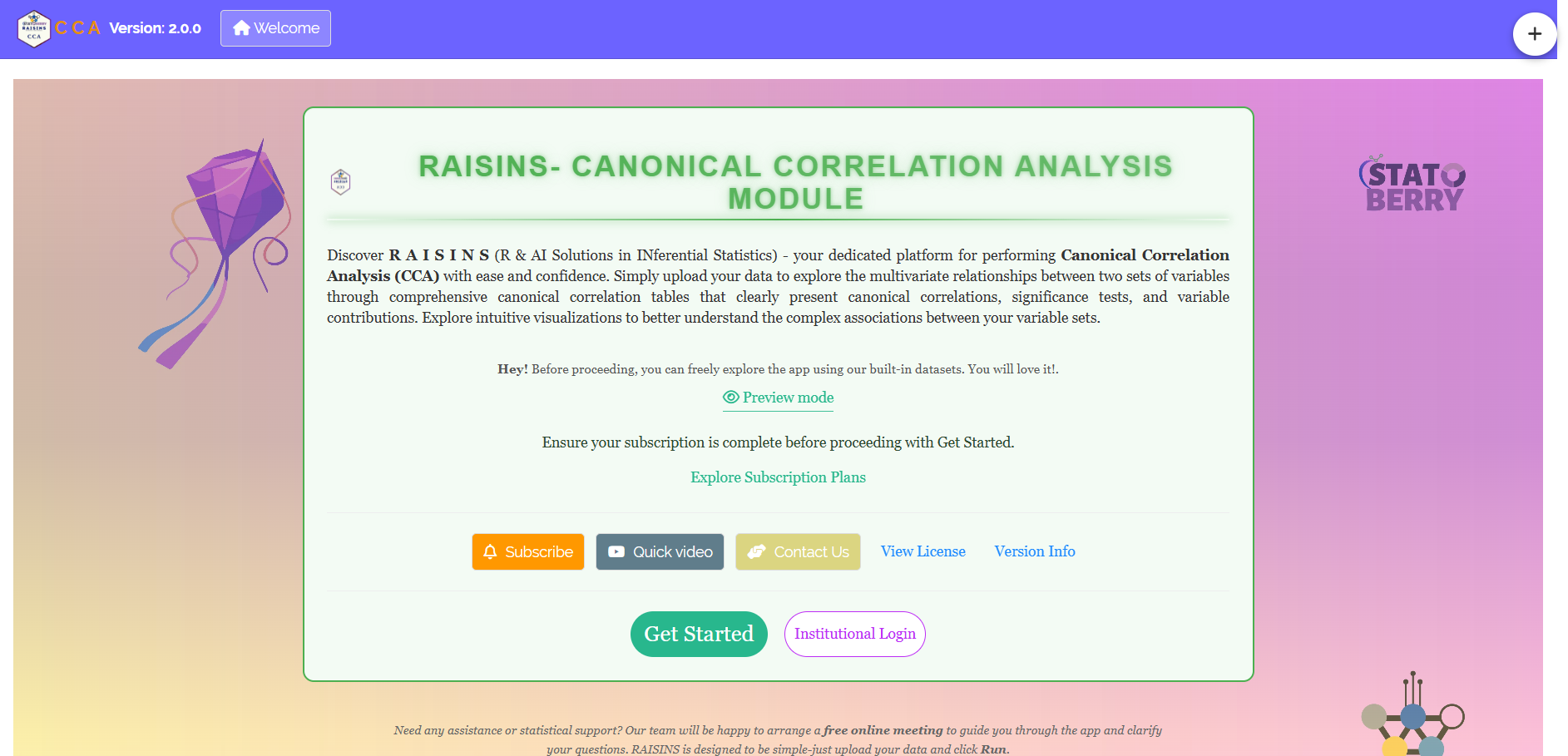
You can explore the entire module before subscribing by using Preview mode on the Welcome page. It loads built-in datasets, so you can try every feature, including the analysis and the plots, without uploading your own data.
First-time users are also offered a Quick Tour. This is an interactive, step-by-step walkthrough that highlights each tab and control and explains what it does. You can replay it at any time from the Quick Tour tab in the top navigation.
5 The Example Dataset
This tutorial uses the built-in Plant Growth Conditions and Development dataset, available from the Datasets tab, covering 55 experimental plots.
The X-set (growing conditions) has four variables:
- Temperature
- Sunlight
- Water
- Fertilization
The Y-set (development outcomes) has four variables:
- Height
- Leaf Count
- Biomass
- Flower Count
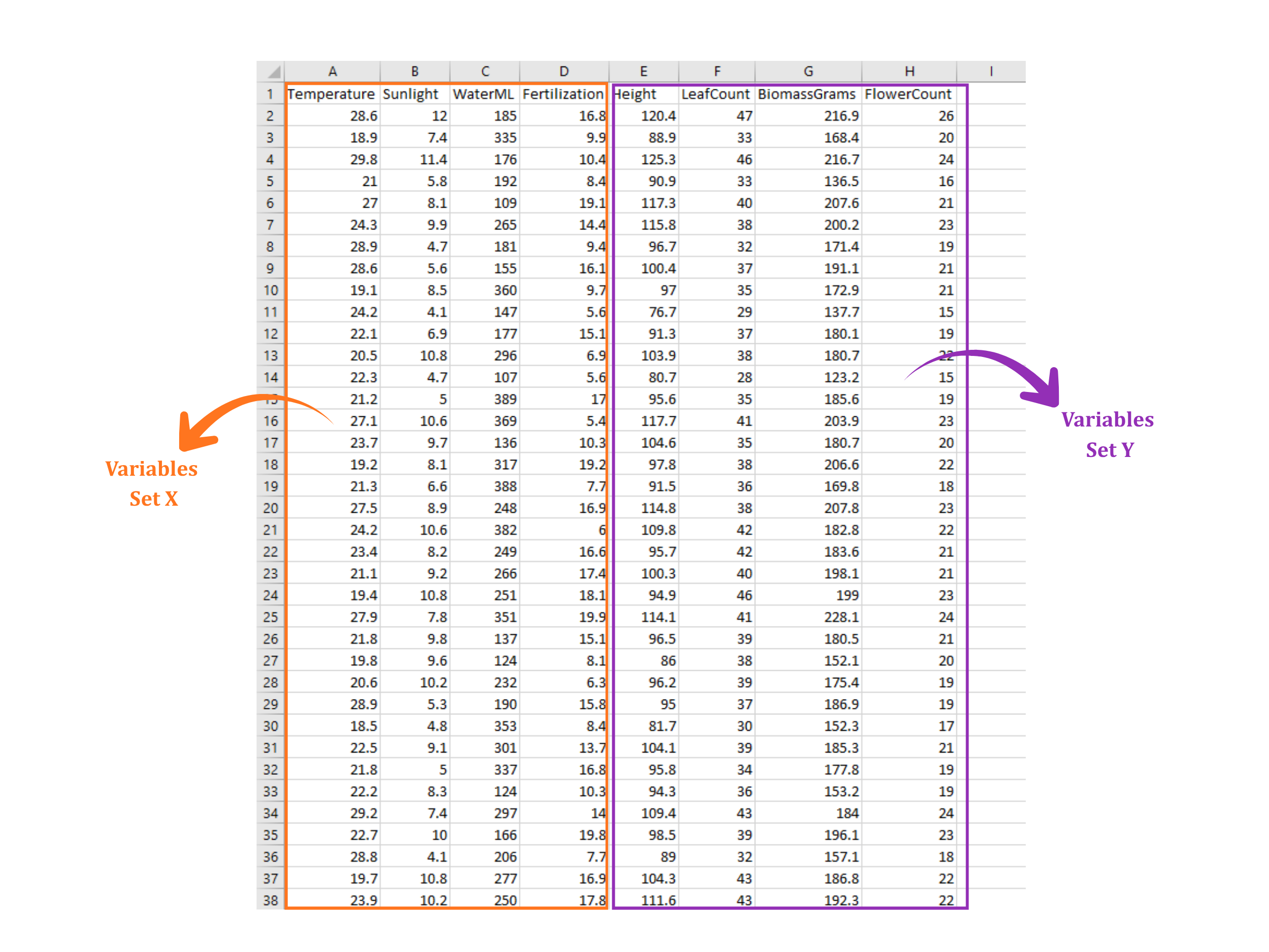
The objective is to find out whether, and how, growing conditions as a whole relate to plant development as a whole. The data layout is shown in Figure 3.
- Prepare your dataset.
- Upload the data.
- Select the X-set and Y-set variables.
- Run the analysis.
- Examine the canonical correlations and Wilks’ Lambda table.
- Review the loading and cross-loading tables.
- Review the plots.
- Read the automatic interpretation, or ask RA-One.
- Export the tables, figures, and the downloadable report.
The sections below walk through each of these steps in detail.
6 Preparing Your Data
The quality of your analysis depends on the quality of your data. RAISINS provides four ways to prepare a correctly formatted dataset:
- Create it in MS Excel.
- Build it inside the app using Create Data.
- Download a built-in Model dataset and use it as a reference.
- Generate it through the RA-One chat assistant.
6.1 Preparing Data in MS Excel
Open a new Excel workbook containing a single sheet. Arrange the data in columns: one column for each X-set variable, and one column for each Y-set variable. Each row represents one observation. Every X-set and Y-set column must contain only numeric values.
Save the file in CSV, XLS or XLSX format. CSV is recommended because it is smaller and loads faster. Avoid blank rows above the data and extra spaces in column names. Refer to Figure 3 for the required layout.
Dataset creation rules
- Column naming - do not use spaces. Use underscores (
_) or dots (.), and avoid symbols such as % and #. Always begin a column name with a letter. - Data arrangement - start at the upper-left corner of the sheet. The row above the data must not be blank.
- Cell management - do not type or delete in empty cells. If needed, select them, right-click, and choose Clear Contents.
- Column relevance - give every column a meaningful name, and remove columns you will not analyse.
- Numeric columns only - every X-set and Y-set column must contain only numbers. Entries such as “NA” or ” - ” will cause errors. CCA does not accept categorical variables in either set.
How to save as CSV in MS Excel
- Open your workbook, with the data on a single sheet and correctly arranged.
- File → Save As / Save a Copy, then choose a location.
- Save as type → CSV (Comma delimited) (*.csv).
- Name the file without spaces. Use underscores instead.
- Save.
💡 Tip: before saving, confirm that the data is on the first and only sheet, and that every X-set and Y-set column is numeric.
6.2 Creating Data Inside RAISINS
If you are unsure about the required format, RAISINS can generate a template for you:
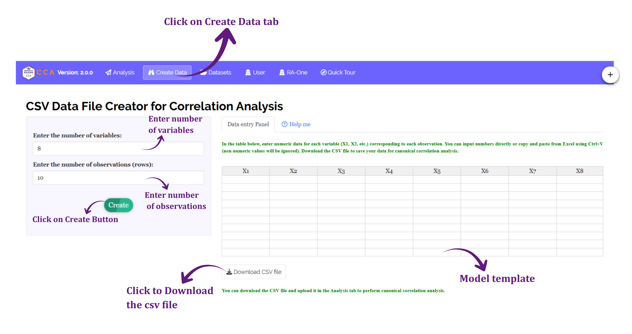
- Go to the Create Data tab.
- Select the number of Variables.
- Select the number of Observations, which is the number of rows.
- Click Create.
The generated layout is shown in Figure 4. Enter your values in the template directly or download the template as a CSV file and enter the values in the downloaded CSV file, then upload it in the Analysis tab.
6.3 Downloading Model Datasets
To explore the module before using your own data, download a ready-made example:
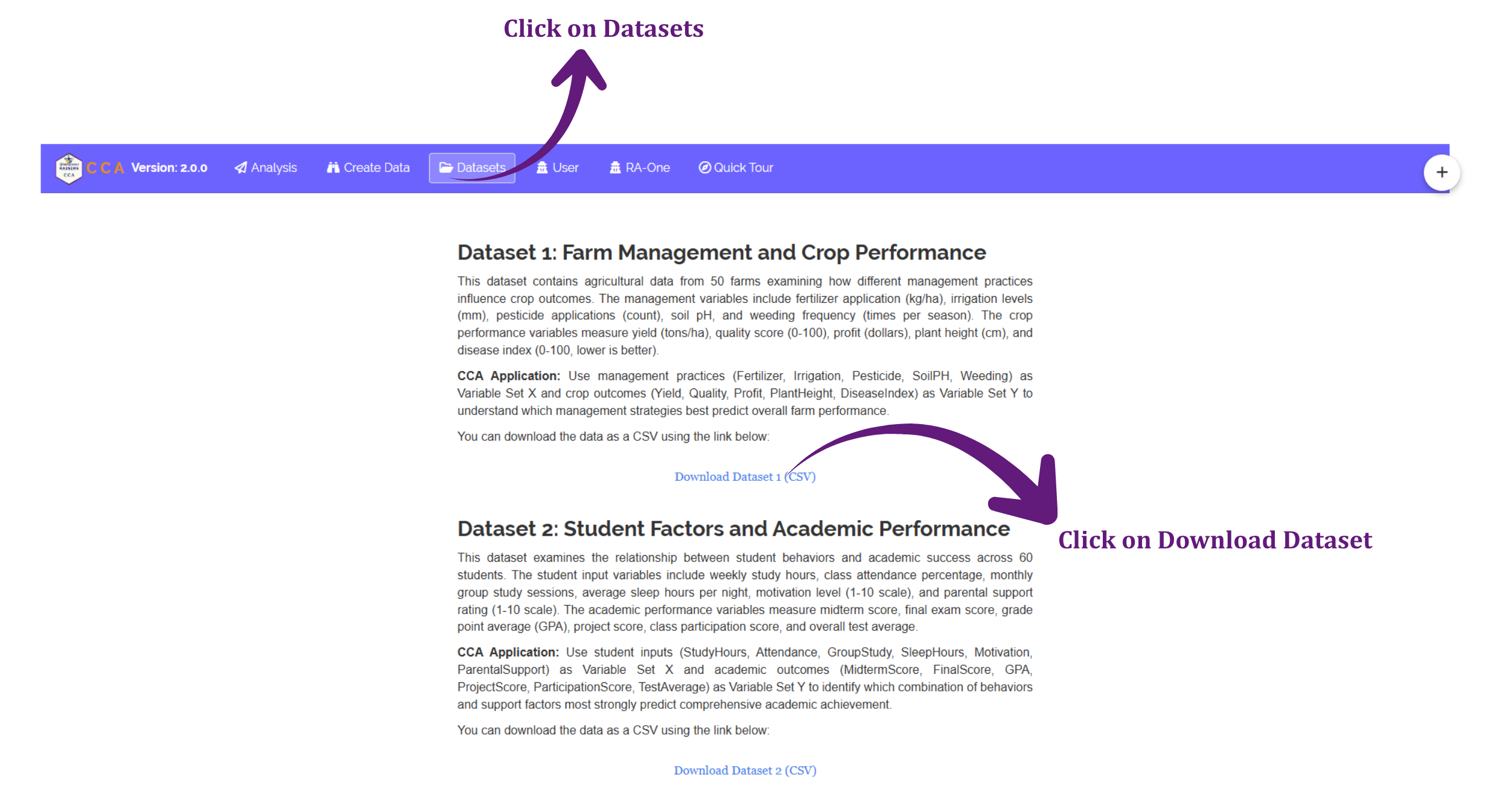
- Go to the Datasets tab.
- Click the Download CSV link for the dataset you want.
- Use it as a formatting reference, or upload it directly to run the analysis.
6.4 Creating a Dataset Using RA-One
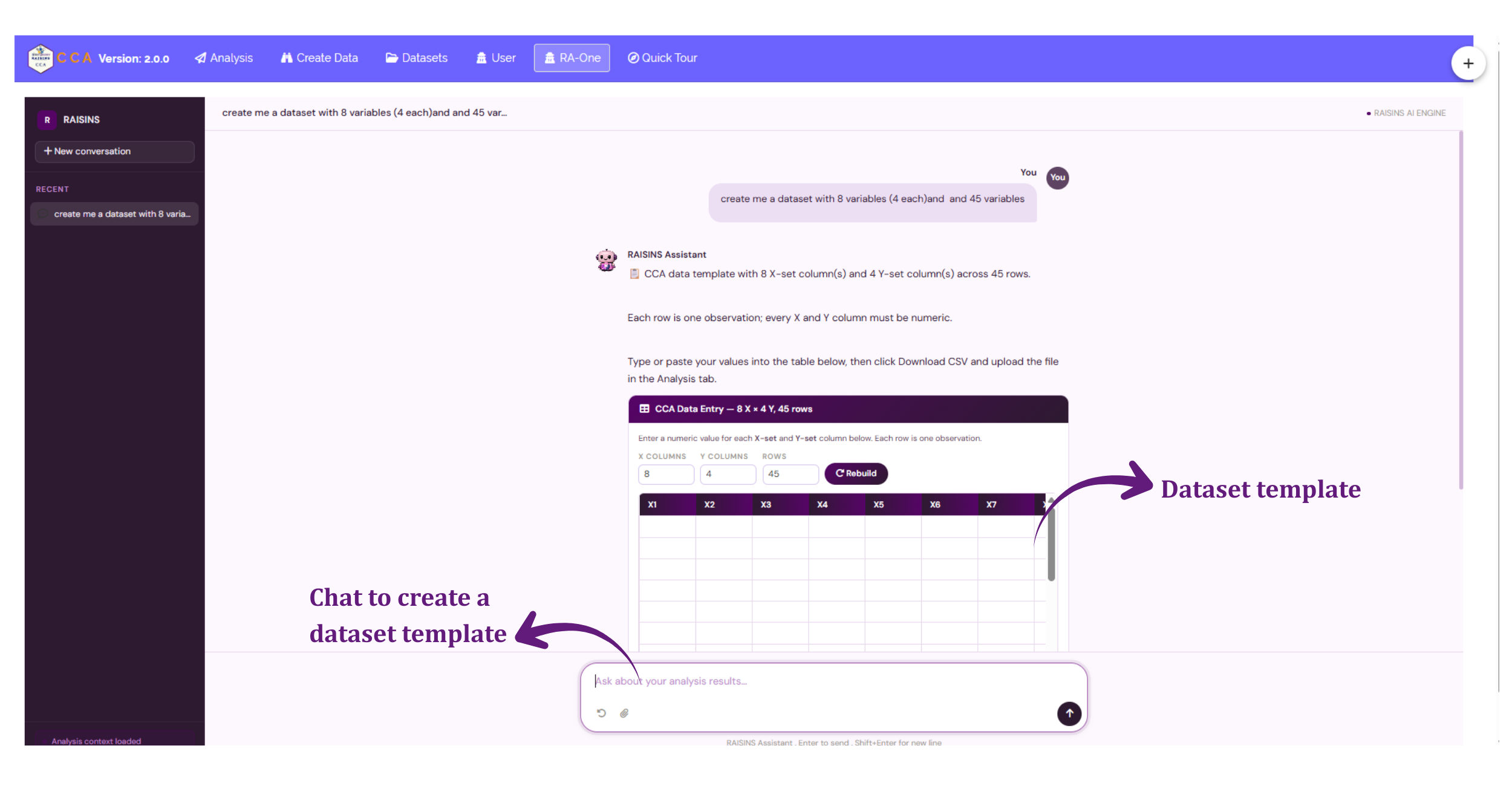
RA-One, the built-in chat assistant, can create a correctly formatted dataset through a simple conversation.
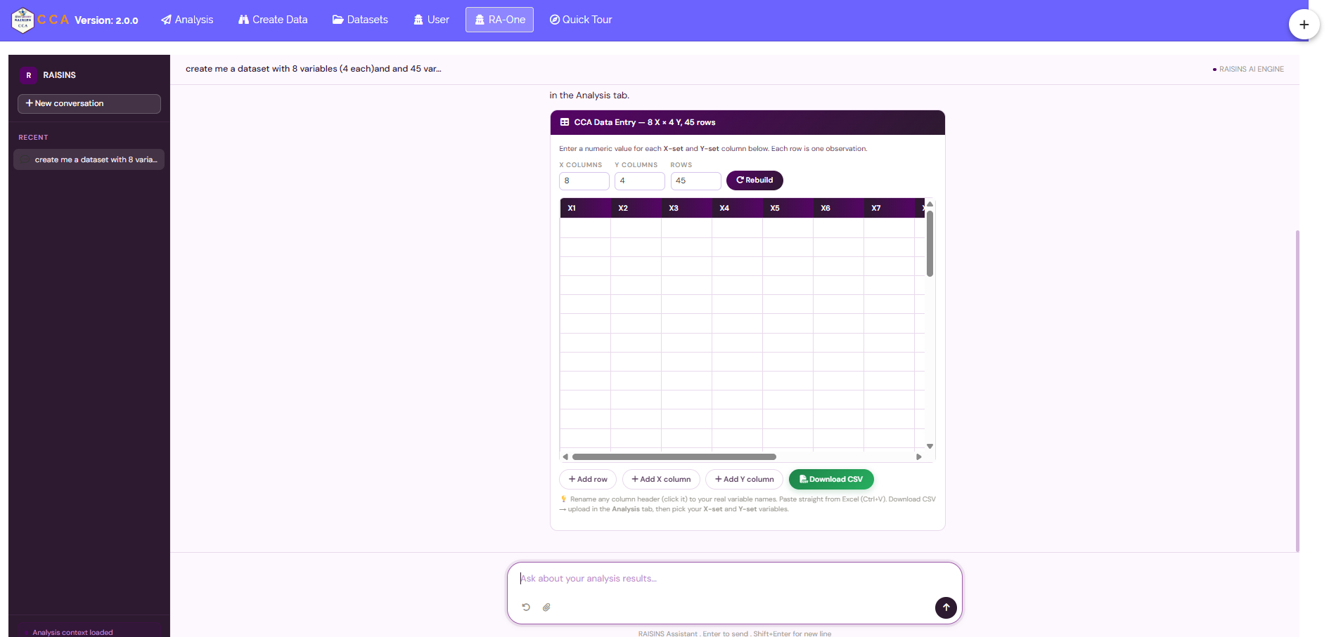
Open RA-One from its navigation tab or from the floating chat bubble. Tell it how many X-set columns, how many Y-set columns, and how many observations you need, and it generates a template in the required format. Review the template in the chat, download the CSV file, and upload it in the Analysis tab (Figure 6).
7 The Analysis Tab
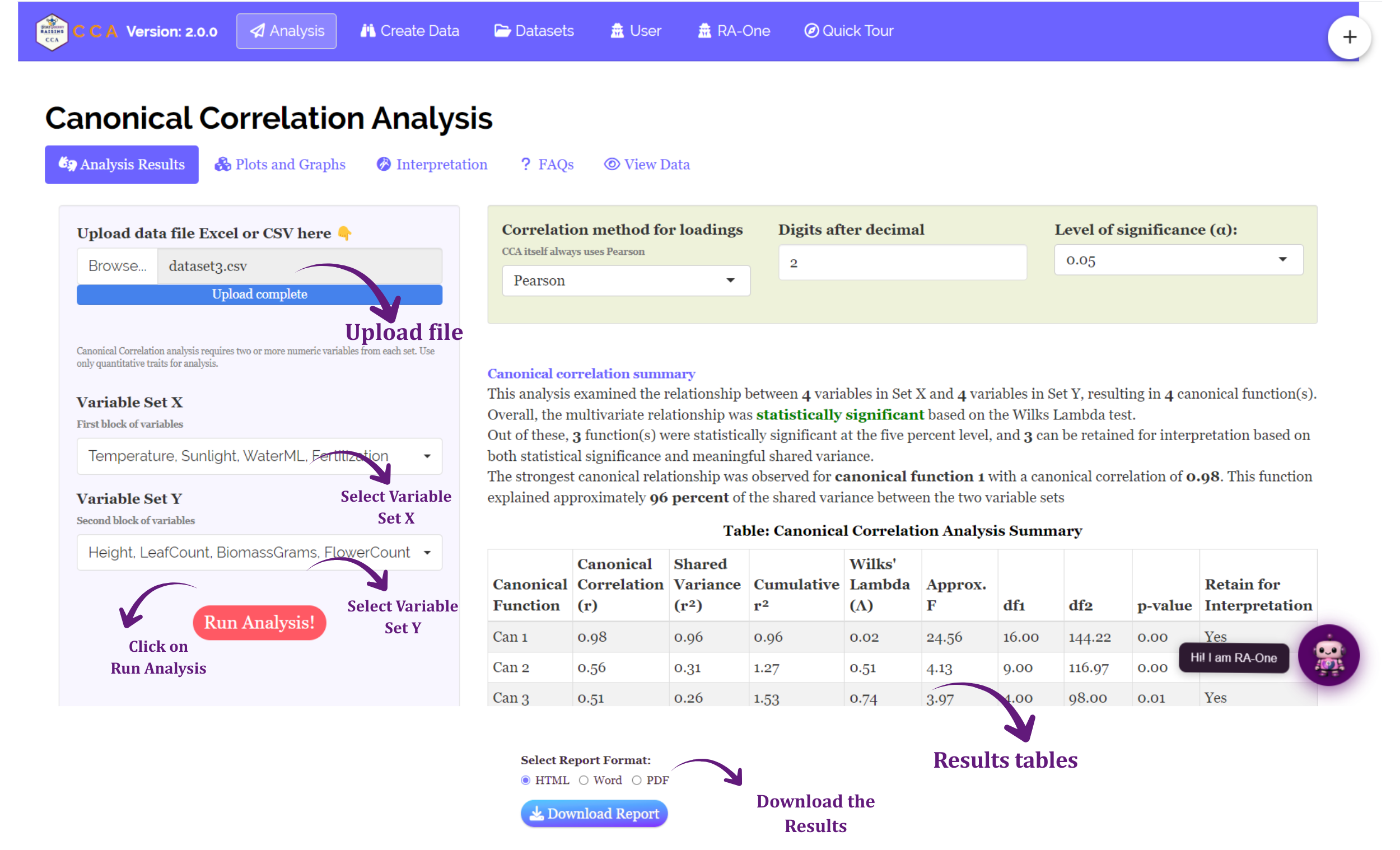
The Analysis tab, under its Analysis Results sub-tab, is where the canonical correlation model is fitted (Figure 7).
Click Browse in the sidebar to upload your CSV or Excel file. Two selectors then appear:
- X-set variables - select at least two numeric columns.
- Y-set variables - select at least two numeric columns. A variable chosen for one set is automatically removed from the choices for the other.
Click Run Analysis. The results appear immediately across the sub-tabs: Analysis Results, Plots and Graphs, Interpretation, RA-One. You can also set the number of decimal digits used in the output tables, and choose the Level of significance (α) - 0.05 or 0.01 - used for the Wilks’ Lambda test and the “Retain for Interpretation” column (see Section 2). Both update the displayed results immediately, without needing to click Run Analysis again.
Unlike a simple correlation, canonical correlation analysis is only meaningful when each side has two or more variables. With a single variable on each side, the “canonical correlation” would simply reduce to an ordinary Pearson correlation.
8 Analysis Results
The Analysis Results sub-tab presents seven tables: the Canonical Correlation Analysis Summary, the raw canonical coefficients for the X-set and Y-set, the canonical loadings for each set against its own canonical variate, and two cross-loading tables. This tutorial refers to them as Table 1 through Table 7, in the order they appear on screen, purely for ease of reference.
The tables are not numbered on screen. RAISINS captions the first table simply “Table: Canonical Correlation Analysis Summary” (no numeral), and the remaining six carry no “Table” prefix at all — just their bare name (for example, “Raw Canonical Coefficients (Set X)”). The “Table 1” through “Table 7” labels used throughout this section are this tutorial’s own numbering, added for readability, not text you will see in the app itself.
Tables 6 and 7 are both cross-loading tables, but only one says so. Each correlates one set’s original variables with the other set’s canonical variate. RAISINS captions Table 7 “Cross Loadings: Y with U” but captions Table 6 “Canonical Loadings: X with V”, not “Cross Loadings: X with V”. This is simply how the two tables are labelled in the app; both are read the same way, as described under Tables 6 and 7 below.
8.1 Table 1: Canonical Correlation Analysis Summary
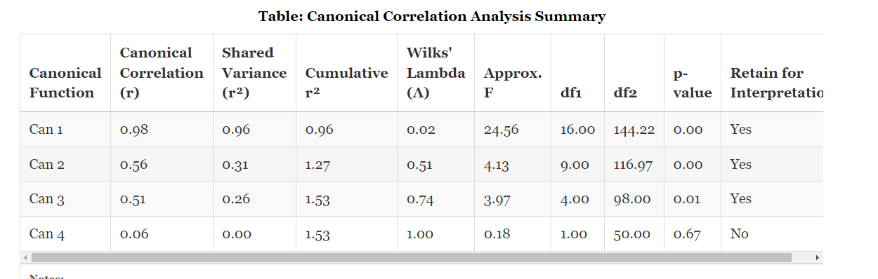
For every canonical function, this table reports the canonical correlation (r), its shared variance (r-squared), the cumulative r-squared across functions up to and including this one, the Wilks’ Lambda statistic, its F-approximation, both degrees of freedom, and the p-value. A final column marks whether the function should Retain for Interpretation, using the rule from Section 2.
Understanding the correlations table
| Column | Meaning |
|---|---|
| Canonical Correlation (r) | The canonical correlation for this function: the correlation between its X-side and Y-side canonical variates |
| Shared Variance (r-squared) | r squared - the proportion of variance the two canonical variates share |
| Cumulative r-squared | The running total of shared variance across this function and every function before it |
| Wilks’ Lambda (Λ) | The test statistic for the sequential significance test of this function through the last one. Smaller values indicate stronger association |
| Approx. F | Rao’s F-approximation to the Wilks’ Lambda distribution, used to obtain the p-value |
| df1 / df2 | Degrees of freedom for the F-approximation |
| p-value | The probability of a Wilks’ Lambda this small if there were truly no relationship remaining in this and all later functions |
| Retain for Interpretation | “Yes” only when p is below the selected significance level (α, 0.05 by default) and r-squared ≥ 0.10 |
Interpretation of Figure 8
For the example dataset, four canonical functions were extracted (p = q = 4). At 4 decimal digits, the results are:
| Function | r | r-squared | Cumulative r-squared | Wilks’ Lambda | Approx. F | df1 | df2 | p-value | Retain |
|---|---|---|---|---|---|---|---|---|---|
| 1 | 0.9822 | 0.9647 | 0.9647 | 0.0180 | 24.5552 | 16 | 144.2250 | 0.0000 | Yes |
| 2 | 0.5571 | 0.3104 | 1.2751 | 0.5108 | 4.1316 | 9 | 116.9700 | 0.0001 | Yes |
| 3 | 0.5066 | 0.2566 | 1.5317 | 0.7407 | 3.9681 | 4 | 98.0000 | 0.0050 | Yes |
| 4 | 0.0605 | 0.0037 | 1.5354 | 0.9963 | 0.1835 | 1 | 50.0000 | 0.6702 | No |
Three of the four canonical functions are retained. The first is overwhelming: r = 0.98, meaning the best combination of growing conditions and the best combination of development outcomes share 96.5% of their variance. Functions 2 and 3 are statistically significant and each clears the 10% shared-variance bar, so they represent real, additional, independent dimensions of relationship, though both are far weaker than the first. Function 4 is neither significant (p = 0.6702) nor practically meaningful (r-squared = 0.0037) and is correctly excluded from interpretation, even though it was mechanically extracted along with the others.
Note that the cumulative r-squared column does not represent a single meaningful “total” the way it might for, say, cumulative variance explained in PCA - each canonical function captures a separate, orthogonal dimension of relationship, so the running sum is provided as a convenience for seeing how much of the four functions’ combined shared variance is concentrated in the earliest, strongest ones (here, over 96% of it sits in Function 1 alone).
At the default 2-digit setting, Function 1’s p-value rounds to a bare 0.00 rather than a true zero; RAISINS reports the exact value computed by CCP::p.asym(), not a special “less-than” notation, so increasing the digit count (as shown here) reveals how small it actually is.
8.2 Tables 2 and 3: Raw Canonical Coefficients (Set X) and (Set Y)
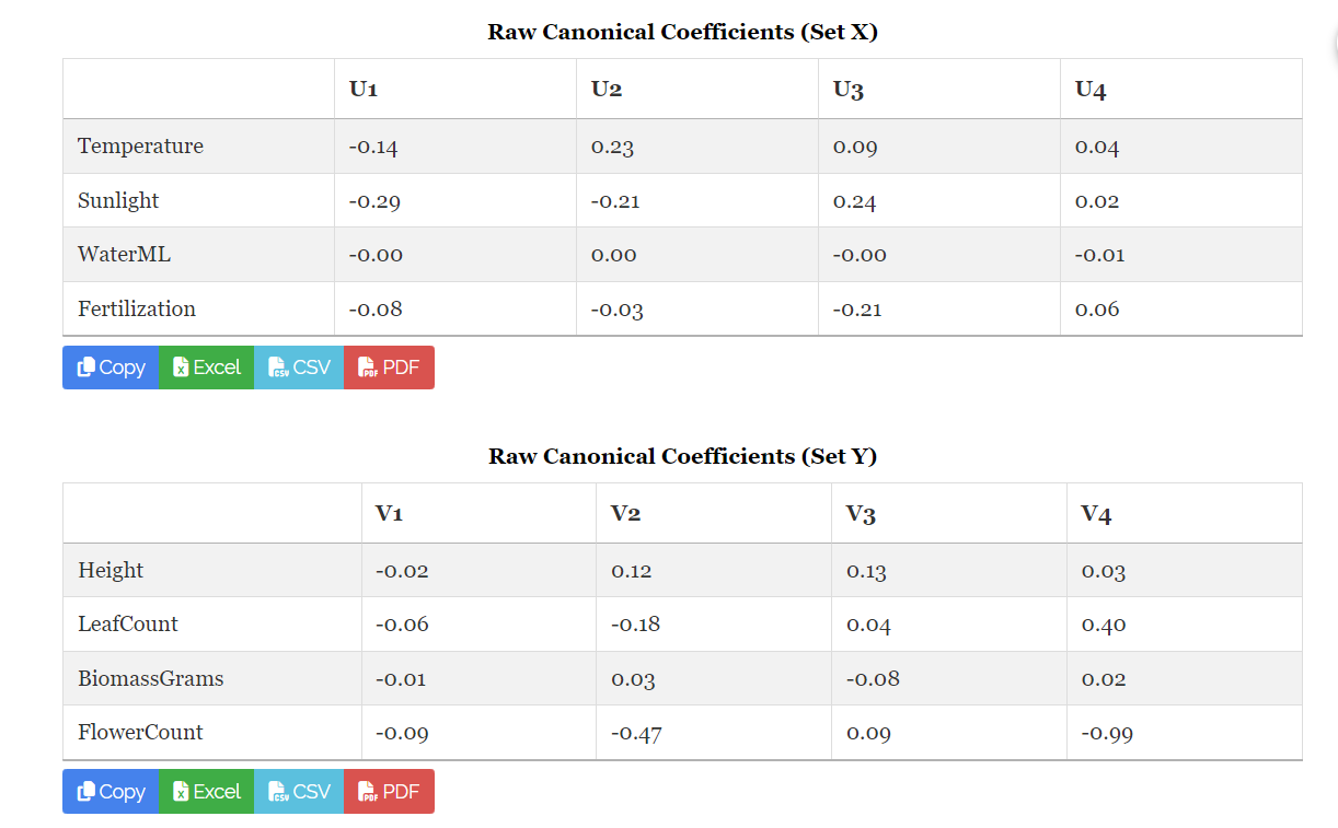
These two tables report the raw canonical coefficients - the weights that define each canonical variate as a linear combination of the original variables. Table 2 covers the X-set (columns U1, U2, …) and Table 3 covers the Y-set (columns V1, V2, …).
Raw coefficients are on a standardized scale and are rarely interpreted variable-by-variable, because their size depends on the scale and correlations among all the variables in that set at once. Use them only if you need the literal formula for a canonical variate. To see which variables actually matter, use the canonical loadings instead.
8.3 Tables 4 and 5: Canonical Loadings (X with U) and (Y with V)
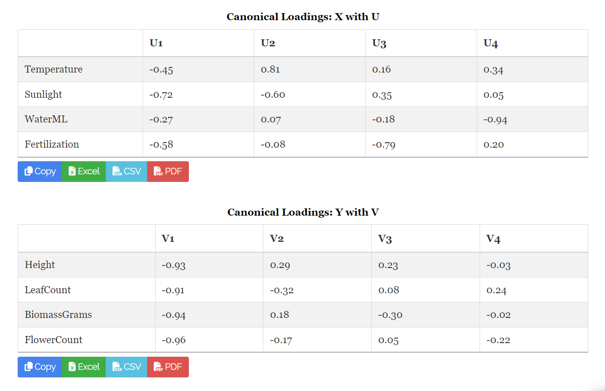
A canonical loading (also called a structure loading) is the correlation between one original variable and the canonical variate built from its own set. Table 4 reports the X-set loadings against U, and Table 5 reports the Y-set loadings against V. RAISINS treats any loading with an absolute value greater than 0.3 as an important contributor to that function.
Interpretation of Figure 10
For the first, dominant canonical function, the X-set loadings on U1 (Table 4) are Temperature -0.45, Sunlight -0.72, WaterML -0.27, and Fertilization -0.58. Using the 0.3 threshold, Sunlight, Fertilization and Temperature are the important contributors; WaterML contributes comparatively little to this function.
The Y-set loadings on V1 (Table 5) are Height -0.93, LeafCount -0.91, BiomassGrams -0.94, and FlowerCount -0.96. Every development outcome loads strongly on this function. In other words, the first canonical function is essentially a single “overall growing conditions” axis (mainly light, fertilization and temperature) tied to a single “overall vigor” axis on which every development measure moves together.
Every loading here has the same sign on each side. Because the canonical correlation itself is positive, consistent signs mean growing conditions and development outcomes rise and fall together: plots with more sunlight, fertilizer and warmth tend to be taller, leafier, heavier and more floriferous, and vice versa. The sign pattern itself has no meaning beyond this consistency, CCA does not fix the direction of a canonical variate.
Two X-set variables that are themselves correlated with each other can “compete” for the same raw coefficient, sometimes leaving one with a small or even sign-flipped weight despite being genuinely important. The canonical loading, being a simple correlation with the canonical variate, does not have this problem, which is why RAISINS’ own interpretation and RA-One both reason from loadings rather than raw coefficients.
8.4 Tables 6 and 7: Canonical Loadings: X with V, and Cross Loadings: Y with U
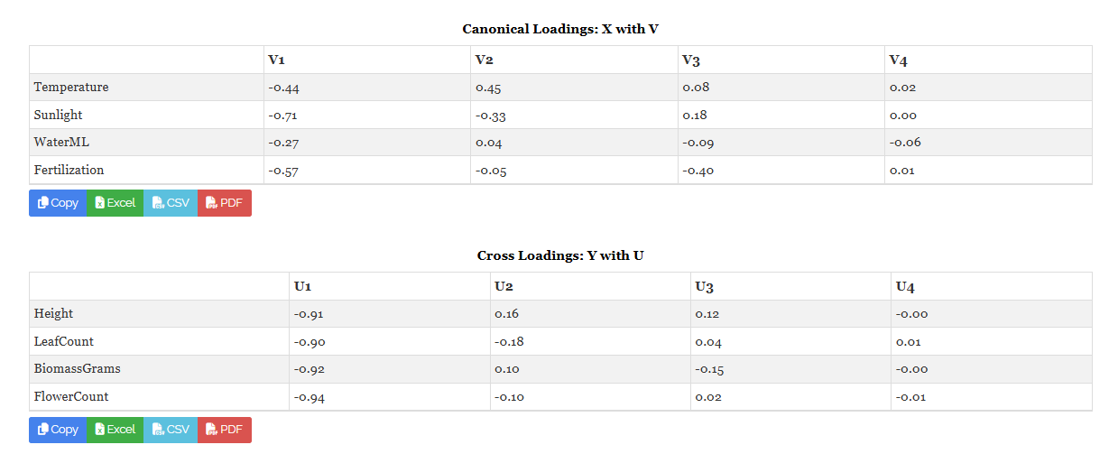
Table 6 (“Canonical Loadings: X with V”) and Table 7 (“Cross Loadings: Y with U”) are both cross-loading tables: each reports the correlation between one set’s original variables and the other set’s canonical variate. They show how strongly a variable relates to the pattern found on the opposite side, not merely to its own set’s own composite.
Cross-loadings are always smaller in magnitude than the corresponding canonical loadings for a given function, because they are attenuated by the canonical correlation itself: a cross-loading is approximately the structure loading multiplied by r for that function. When r is high, as it is for Function 1 here, the two are close; when r is low, the cross-loadings shrink toward zero even for variables with strong canonical loadings.
Canonical correlation analysis describes an association between two sets of variables in the data provided. It does not, by itself, establish that one set causes changes in the other. Treat the result as evidence of a relationship, not proof of cause and effect, unless the study design specifically supports a causal claim.
9 Plots and Graphs
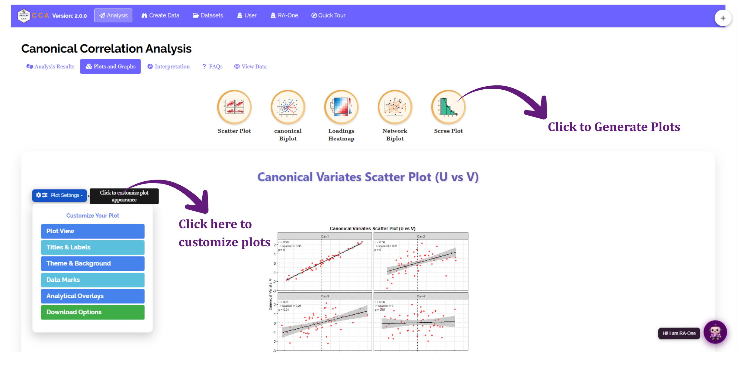
The Plots & Graphs tab contains five visualizations. Select a plot using the row of icon buttons. The selected plot appears below, with a gear icon (Plot Settings) in the corner for customization.
Every plot can be customized. You can change the title, the axis labels, the colours, the point size and the theme. Every plot can also be downloaded, at a resolution you choose.
Hover over any thumbnail below to see what it displays.
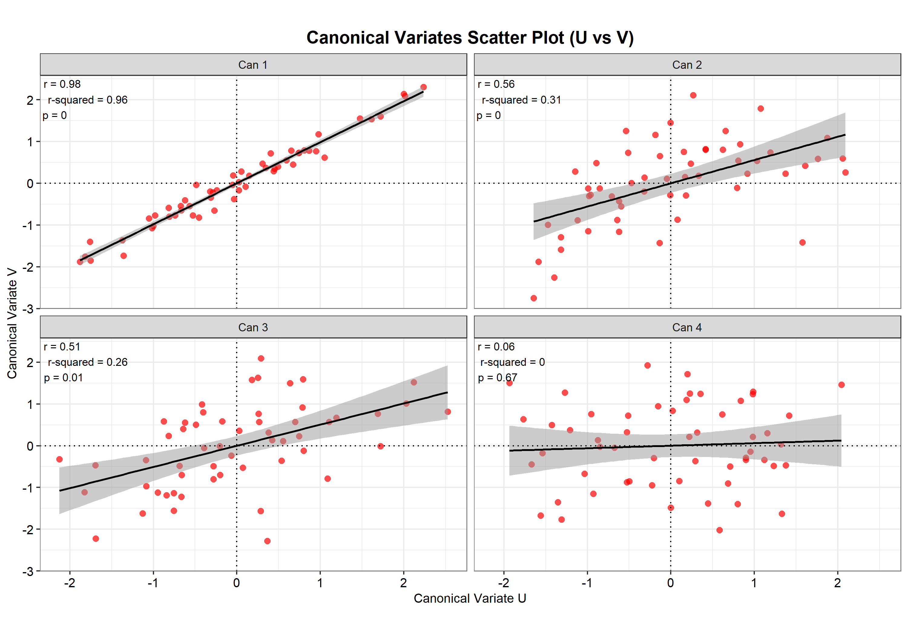
Canonical scores plot. The X-side and Y-side canonical variate scores plotted against each other, one panel per function. Shows how tightly U and V actually track each other.
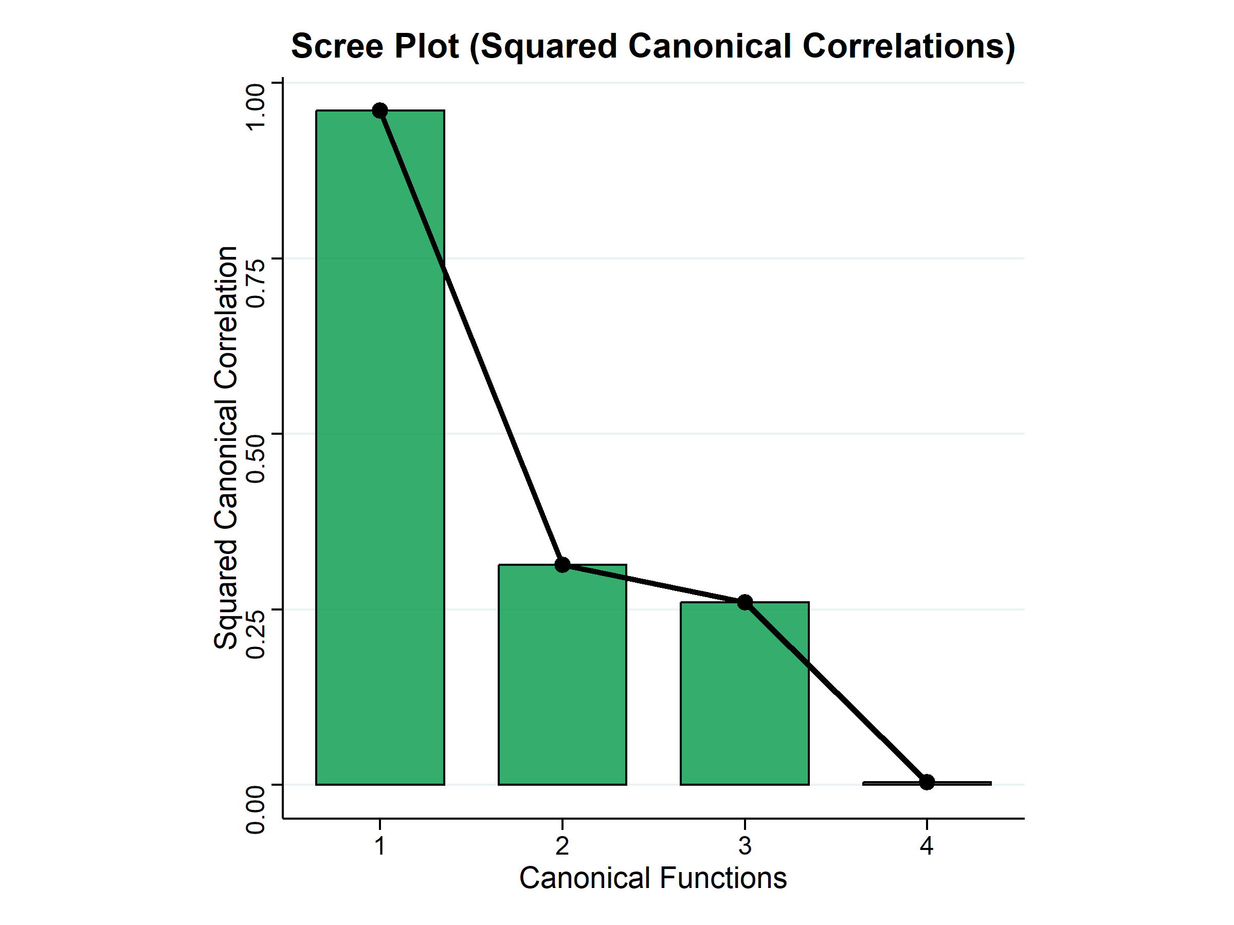
Scree plot. The r-squared (shared variance) of each canonical function, so you can see at a glance how quickly the relationship’s strength drops off after the first function.
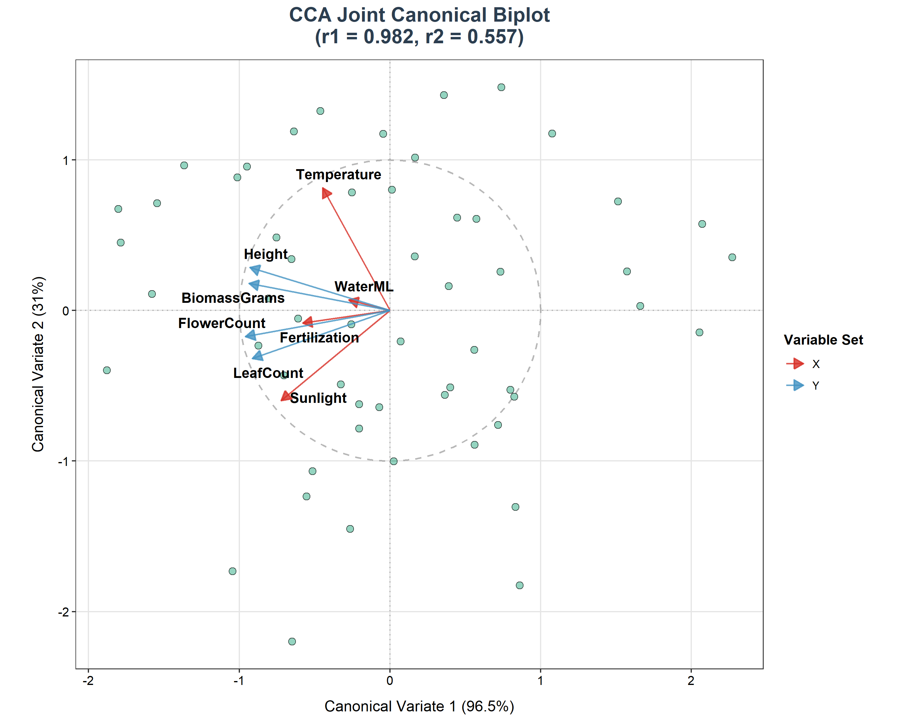
Canonical biplot. Joint observation positions with variable loading arrows on a chosen pair of canonical dimensions, showing which variables pull in which direction.
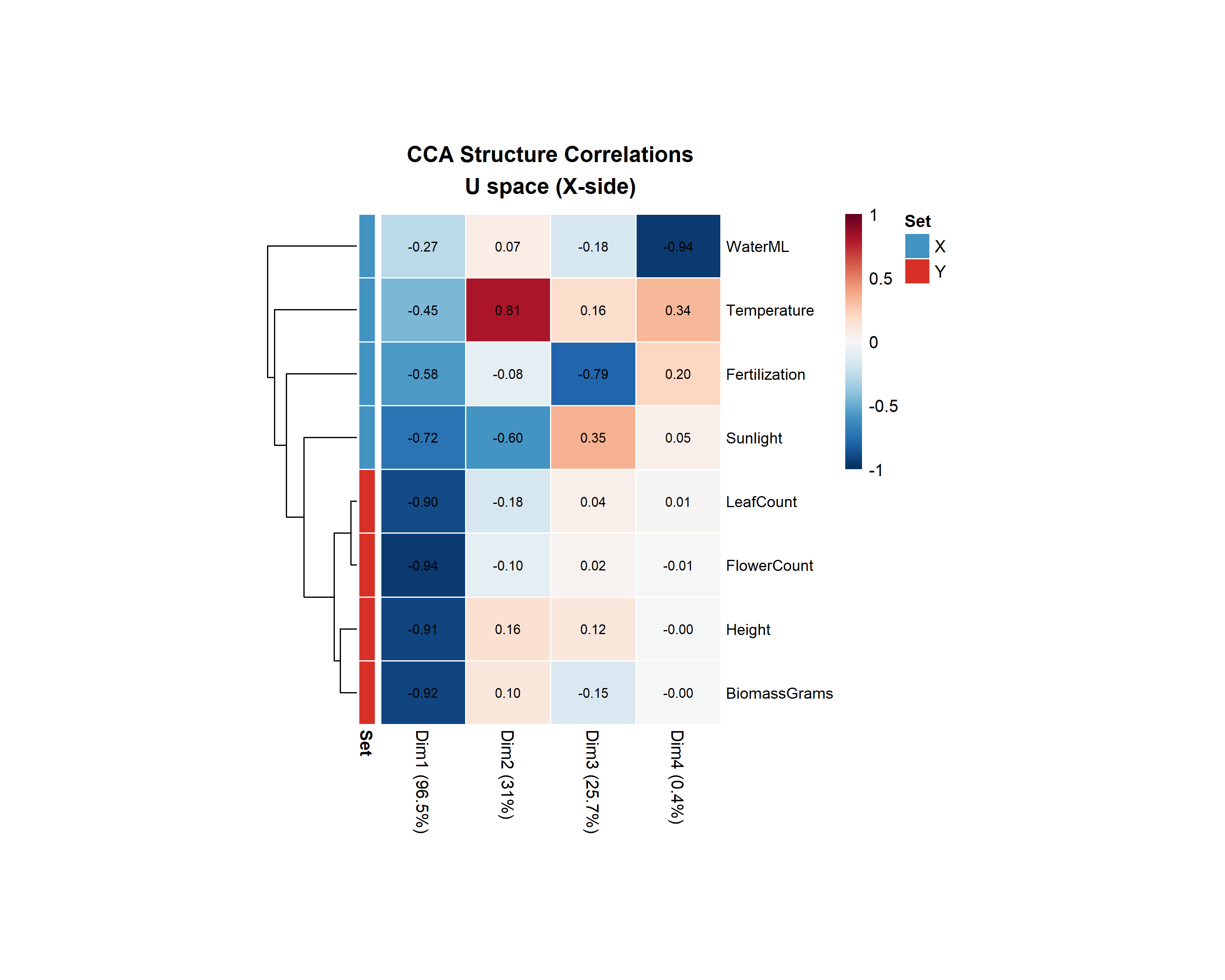
Loadings heatmap. Every structure loading for the X-set and Y-set, coloured by strength and direction, for a quick overview across all functions at once.
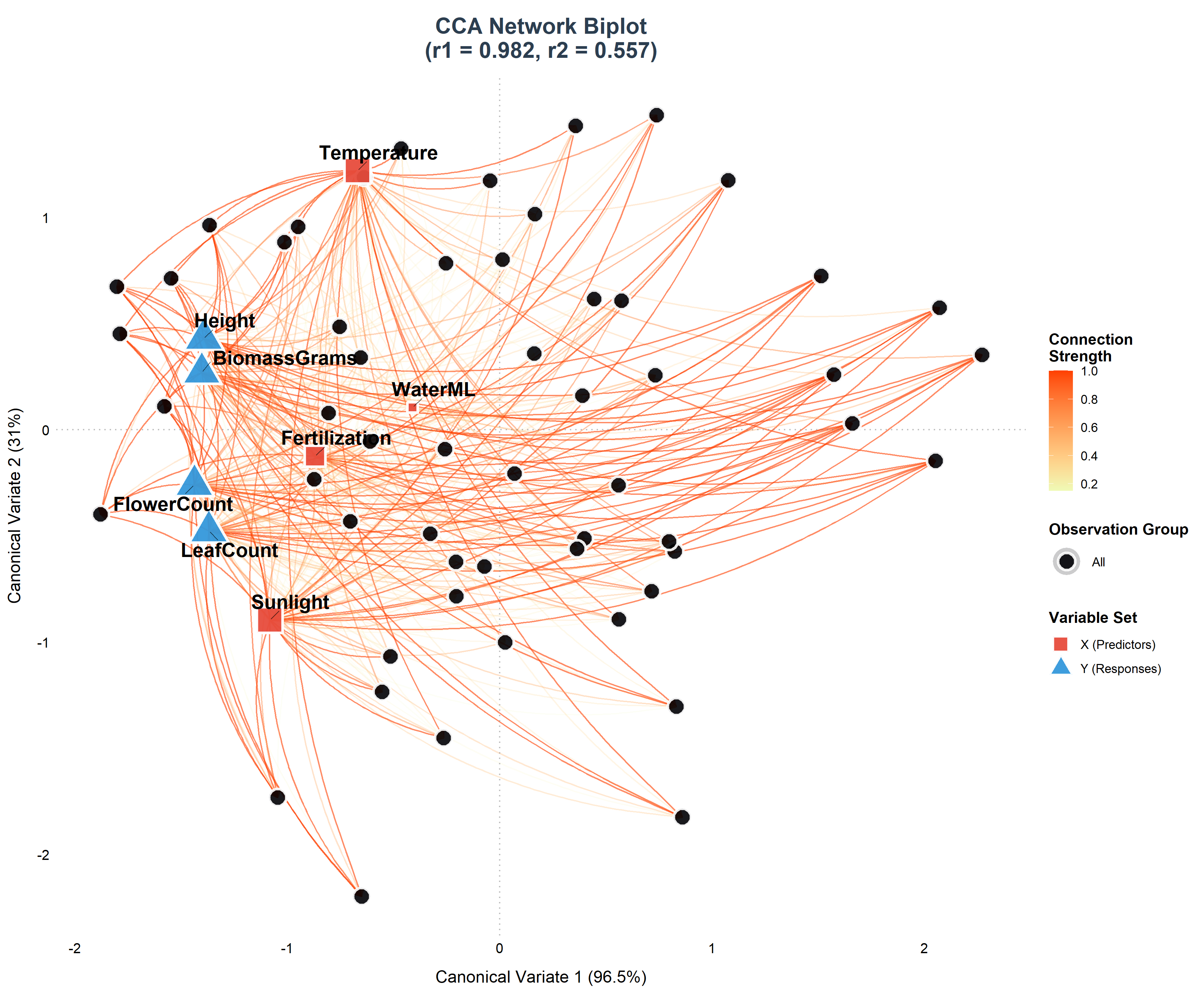
Network plot. Variables positioned by loading strength around a central hub, with only the strongest loadings drawn, at a threshold you can adjust.
10 Interpretation
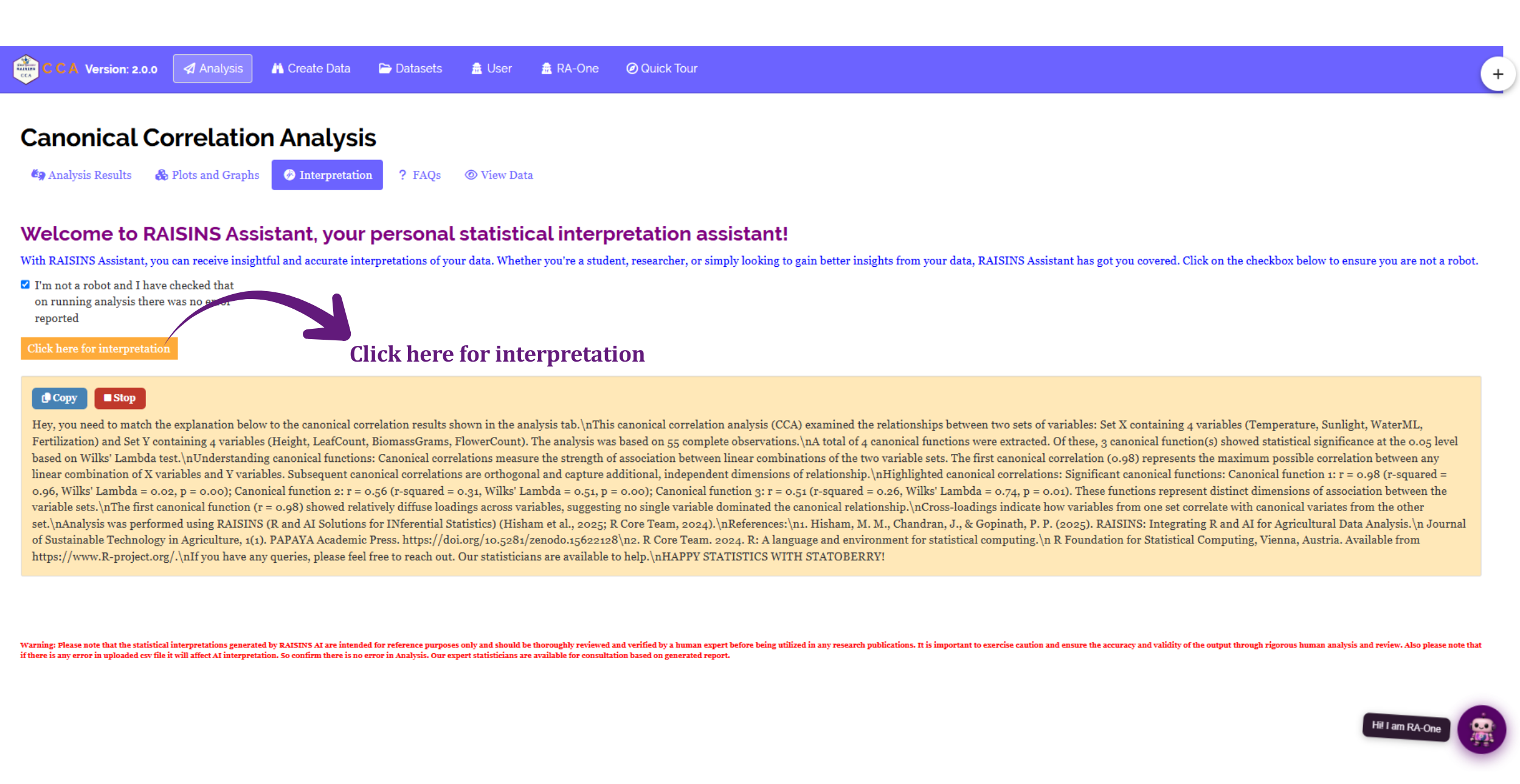
The Interpretation sub-tab provides a written summary of your results in plain language (Figure 18). It reports how many canonical functions were extracted, which are statistically significant, the canonical correlation and r-squared of the leading function, and which X-set and Y-set variables dominate it.
The text appears with a short typing animation. A Stop button displays the full summary immediately, and a Copy button copies the plain-text version to your clipboard.
11 RA-One Chat Assistant
RA-One is the built-in chat assistant. You can open it from its navigation tab or from the floating chat bubble.
Ask questions in plain language, and RA-One answers using your own analysis results. It does not give generic advice, and it does not invent values. If a value is not available, it says so. All replies are in plain English, with no code.
RA-One has access to the complete set of results produced by the app:
- The canonical correlations, r-squared values, and the full Wilks’ Lambda table for every function, including which are retained.
- The structure loadings and cross-loadings for both the X-set and the Y-set.
- The dataset overview: sample size, and the variables in each set.
You can ask it to explain what a canonical correlation, a loading, or the Wilks’ Lambda test means for your specific results. It can also explain the difference between a structure loading and a cross-loading, or why a statistically significant function was not retained for interpretation.
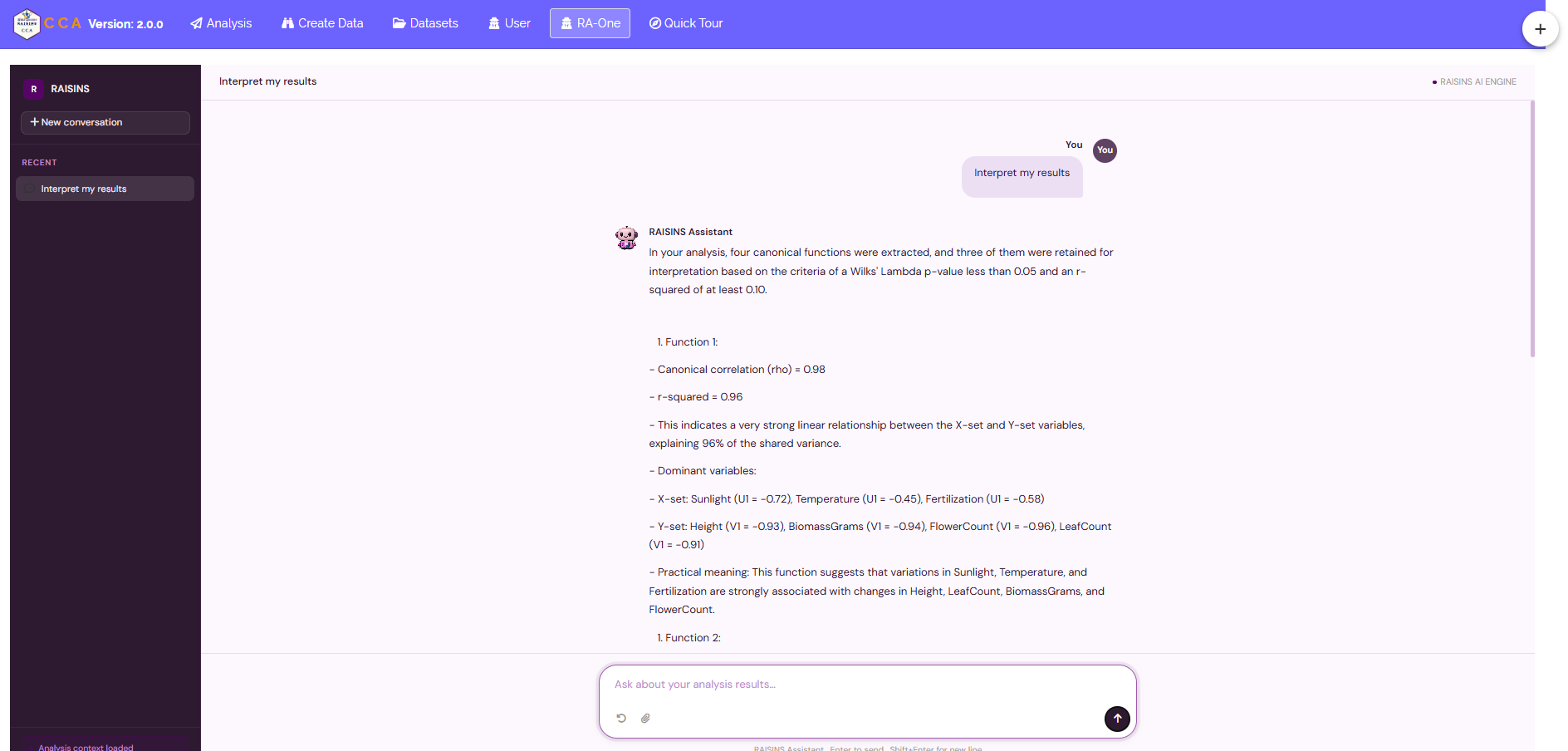
RA-One can also prepare data and generate plots.
It can build a correctly formatted data template (Section 6.4) or provide a model dataset (Section 6.3). It can also create plots on request. For example, you can ask for “the canonical scores plot”, “the scree plot”, “a biplot”, or “the loadings heatmap”, and the figure is displayed directly in the chat.
Each plot created in the chat includes a plot-type toolbar for switching between graph types, a Plot Settings panel for changing the appearance and, for the biplot and network plot, choosing which pair of canonical dimensions to show, and a one-click download.
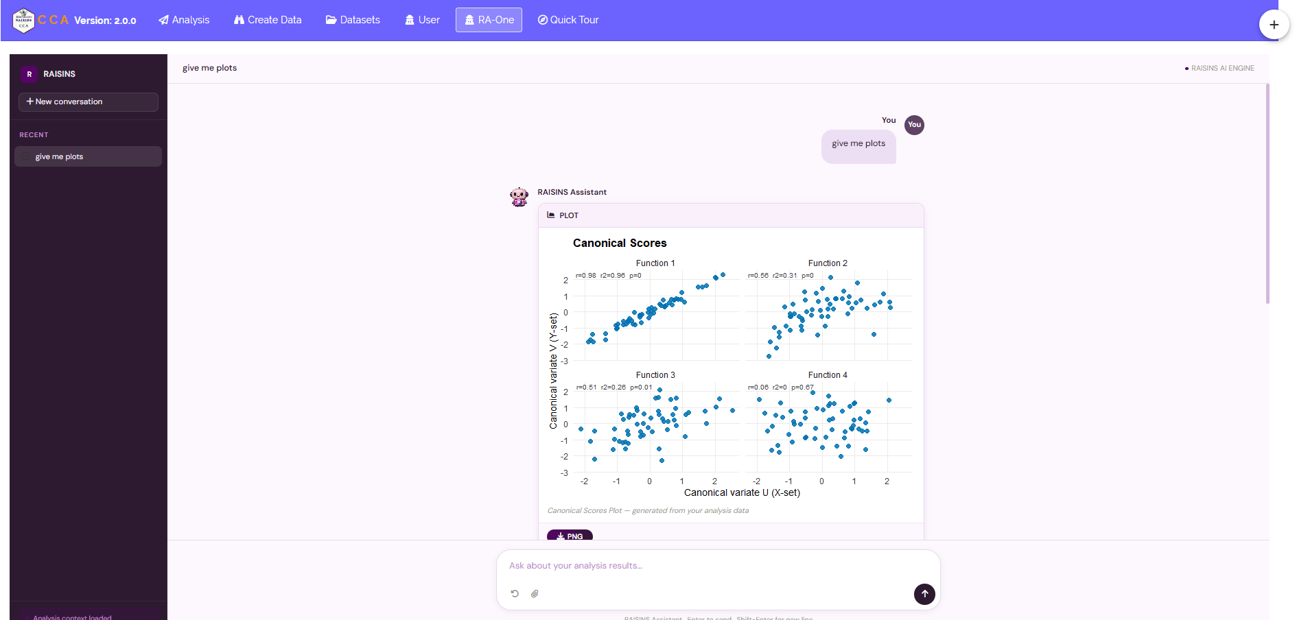
In a single conversation, RA-One can interpret your results, build a data template, provide a model dataset, and create customizable plots. Much of a routine canonical correlation session can be completed without leaving the chat.
12 Downloadable Report
Below the seven results tables in Analysis Results, a Download Report control lets you export the complete set of results as a single document, in HTML, PDF, or Word format (?@fig-report).
The report contains the same Data Summary and Tables 1 through 7 (Canonical Correlation Analysis Summary, Raw Canonical Coefficients, and Canonical/Cross Loadings) shown on screen, so it can be attached directly to a manuscript or shared with a supervisor without needing to copy each table by hand.
13 FAQs
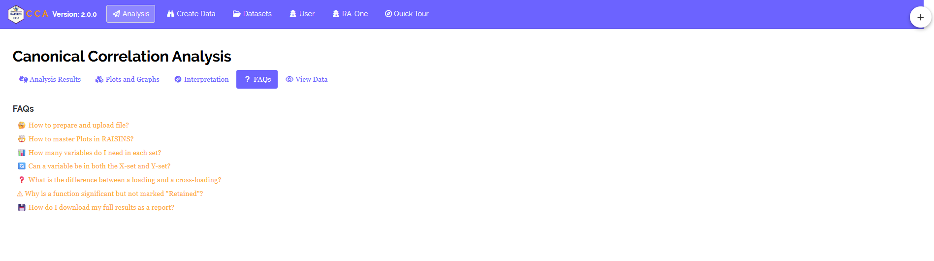
The FAQs tab answers common questions about canonical correlation analysis and about the module itself. It covers topics such as how to choose which variable belongs in the X-set versus the Y-set, what to do when a canonical function is significant but not retained, and how loadings differ from cross-loadings.
If you are unsure how a feature works, start here.
14 View Data
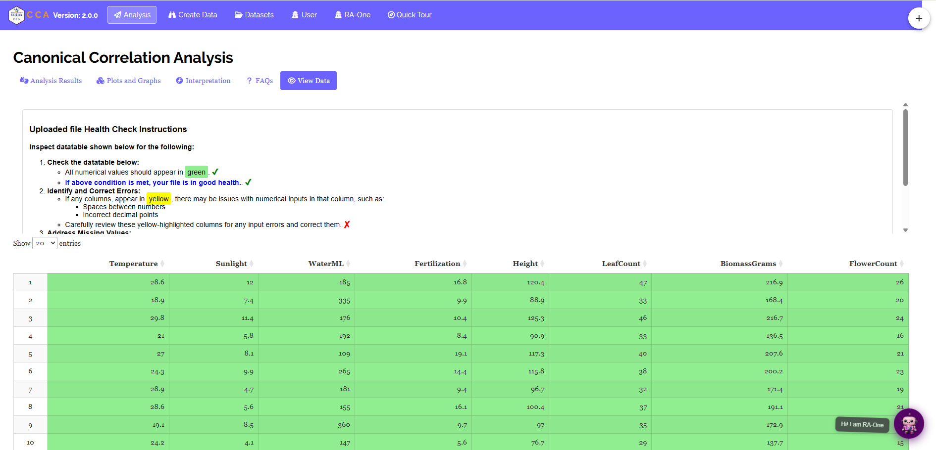
The View Data tab helps you confirm that your dataset is suitable for analysis.
When you upload a file, RAISINS runs an automated Health Check. It examines the column types and formatting, and flags any column that contains non-numeric values, missing entries, or inconsistent formatting.
Resolve any issues reported here before clicking Run Analysis, so that your results are based on clean and correctly formatted data.
15 Summary
Canonical correlation analysis answers a single question: how strongly, and along how many independent dimensions, do two whole sets of variables relate to each other?
Everything else in the output exists to make sure that question is answered correctly and honestly: the Wilks’ Lambda significance test, the practical-retention rule, and the loading and cross-loading tables that separate a genuinely important variable from one merely along for the ride. RAISINS performs all of these calculations automatically, so you can concentrate on interpreting what the results mean for your research.
If you need help at any stage, RA-One is available at all times. You can also write to us at [email protected].
16 Appendix: A Short History of Canonical Correlation Analysis
Canonical correlation analysis was introduced by Harold Hotelling in his 1936 paper “Relations Between Two Sets of Variates”, published in Biometrika. Hotelling, already known for Hotelling’s T² statistic, framed the method as a natural generalization of ordinary correlation: instead of asking how two single variables relate, ask how two whole sets of variables relate, by finding the linear combination of each set that correlates most strongly with the other.
For decades, CCA remained mostly a theoretical tool, computationally demanding relative to the technology of the time and comparatively difficult to interpret without modern software. It became far more practical with the growth of computing power in the second half of the twentieth century, and today it is used across agriculture, ecology, psychology and the social sciences whenever a researcher wants to relate one multivariate battery of measurements to another, such as a set of environmental conditions to a set of growth or performance outcomes.
CCA is also the mathematical ancestor of several later multivariate techniques. Redundancy analysis, and later partial least squares, were both developed to address specific limitations of the original method, but the core idea, finding the pair of composite variables that correlate most strongly, traces directly back to Hotelling’s 1936 paper.
