Exploratory Factor Analysis (EFA)
Exploratory Factor Analysis uncovers the hidden structure behind a set of correlated variables. This tutorial explains factors, loadings, communalities and rotation in plain language, then runs the complete analysis in RAISINS without code, using a reproducible worked example… Read more …
Exploratory Factor Analysis asks a simple question of a wide dataset: are these many measured variables really measuring many different things, or only a few underlying ones? This tutorial explains what a latent factor is, what a loading, a communality and an eigenvalue mean, and how the number of factors is decided. It then works through the complete procedure in RAISINS: preparing the data, choosing an extraction method and a rotation, reading every results table, examining the plots, and using the automatic interpretation and the RA-One assistant. A closing section summarises the pitfalls that most often affect a published factor analysis and shows how the results of this worked example would typically be reported in a thesis or manuscript. Every number shown comes from a real analysis of a dataset built into the module, so the entire tutorial can be reproduced.
1Statoberry LLP, 2Department of Agricultural Statistics, Kerala Agricultural University
1 What is Exploratory Factor Analysis?
Suppose you collected responses from 100 farmers. Each farmer rated a new advisory mobile application on seven usability attributes. You now want to know whether these seven ratings measure seven separate things, or whether the farmers were really responding to a smaller number of broader impressions.
Exploratory Factor Analysis answers this question. It examines the correlations among your measured variables and identifies a smaller set of underlying variables, called factors, that could have produced those correlations. The factors are described as latent because they are never measured directly; they are inferred from the pattern of correlations among the variables you did measure.
Exploratory Factor Analysis gives you two useful pieces of information:
- Structure - It shows which variables group together, and therefore how many distinct constructs your instrument is actually measuring.
- Data reduction - It replaces a large set of correlated variables with a smaller set of factors that retain most of the shared information.
The analysis is called exploratory because you do not specify in advance which variable belongs to which factor. The structure emerges from the data. When you already have a firm, theory-driven hypothesis about the structure, Confirmatory Factor Analysis is the appropriate method instead.
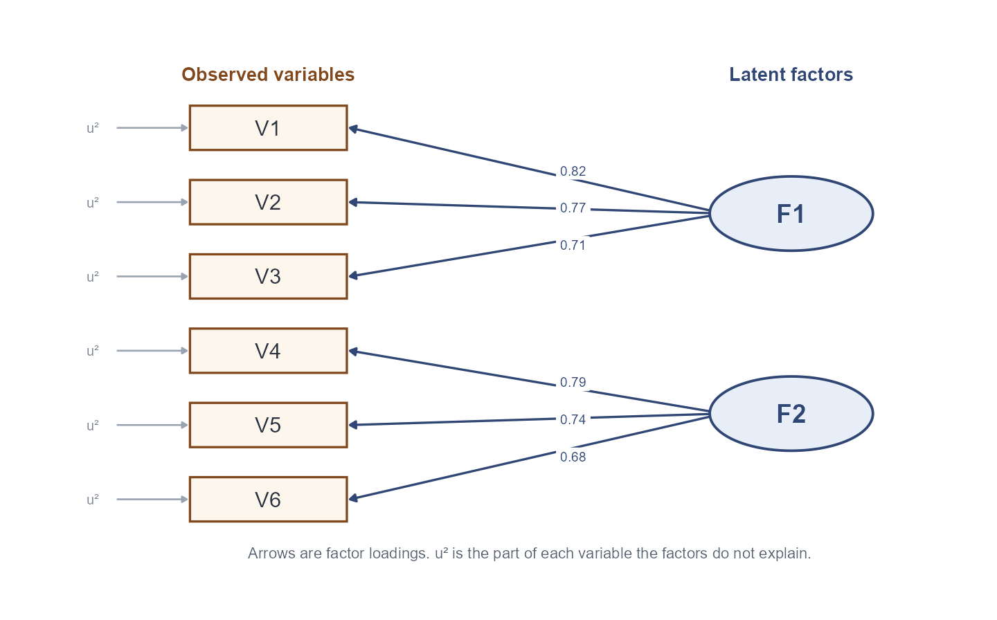
Figure 1 shows the idea for six variables and two factors. Each rectangle is a measured variable. Each ellipse is a latent factor. The arrows are factor loadings, showing how strongly each factor influences each variable. The small arrow entering each variable is its uniqueness, the part of that variable the factors do not explain.
Behind the scenes (optional): the factor model
Most users never need this. Each observed variable is modelled as a weighted sum of the common factors plus a term unique to that variable:
\[X_j = \lambda_{j1}F_1 + \lambda_{j2}F_2 + \cdots + \lambda_{jm}F_m + \varepsilon_j\]
Here \(\lambda_{jm}\) is the loading of variable \(j\) on factor \(m\), and \(\varepsilon_j\) is the unique part of variable \(j\). Written for the whole correlation matrix, the model states that
\[R \approx \Lambda \Phi \Lambda' + \Psi\]
where \(\Lambda\) holds the loadings, \(\Phi\) holds the correlations among the factors, and \(\Psi\) holds the uniquenesses. RAISINS estimates these automatically; no manual calculation is required.
Exploratory Factor Analysis examines the correlations among your measured variables and identifies a smaller number of underlying factors that explain them, showing which variables belong together and how much of each variable the factors account for.
1.1 Exploratory Factor Analysis versus Principal Component Analysis
Because the two methods are frequently confused, and often produce similar-looking output from the same data, the distinction is worth stating clearly before going further.
| Aspect | Exploratory Factor Analysis | Principal Component Analysis |
|---|---|---|
| Question asked | Why do these variables correlate? | How can these variables be summarised in fewer numbers? |
| Variance modelled | Shared (common) variance only | Total variance |
| Underlying assumption | Latent constructs are treated as the cause of the observed correlations | No claim is made about an underlying cause |
| Typical use | Scale development, construct validation, uncovering the structure of a questionnaire | Data reduction before regression, clustering, or plotting |
Use Exploratory Factor Analysis when the aim is to explain why a set of variables correlates and to argue that an underlying construct exists. Use Principal Component Analysis when the aim is simply a smaller number of variables, with no claim about latent causes. The two are not interchangeable in principle, even though they can give numerically similar answers when communalities are high. RAISINS provides a separate module for PCA.
1.2 Reading a Loading
A loading is the correlation between one variable and one factor. It ranges from −1 to +1.
- A large positive loading means the variable increases as the factor increases.
- A large negative loading means the variable decreases as the factor increases.
- A loading near zero means the variable is unrelated to that factor.
By convention, a loading of 0.4 or above in absolute value is treated as meaningful. This threshold is a widely used convention rather than a fixed statistical rule, and a stricter cut-off is sometimes applied in smaller samples, where loadings are estimated less precisely. Variables that load highly on the same factor are interpreted as measuring the same underlying construct, and they determine what that factor is called.
A variable that loads above 0.4 on two or more factors is said to cross-load. Cross-loadings make interpretation ambiguous and often indicate that a different number of factors should be tried.
1.3 Communality and Uniqueness
The communality (h²) of a variable is the proportion of its variance explained by all retained factors together. A communality of 0.83 means the factors account for 83% of what makes that variable vary.
For any variable, the communality is the sum of its squared loadings across the retained factors, and the uniqueness is what is left:
\[h_j^2 = \sum_{m} \lambda_{jm}^2 \qquad\qquad u_j^2 = 1 - h_j^2\]
A communality below 0.3 indicates that the factor solution explains very little of that variable. Such a variable is a candidate for removal, after which the analysis is run again.
1.4 Eigenvalues and Variance Explained
An eigenvalue measures how much total variance a factor accounts for, expressed in units of variables. An eigenvalue of 3.4 means the factor explains as much variance as roughly three and a half of the original variables. It is obtained by summing the squared loadings down a factor column, and dividing by the number of variables converts it into a proportion of the total variance:
\[\text{Eigenvalue}_m = \sum_{j} \lambda_{jm}^2 \qquad\qquad \text{Proportion of variance}_m = \frac{\sum_{j} \lambda_{jm}^2}{p}\]
Because each standardised variable has a variance of exactly 1, a factor with an eigenvalue above 1 explains more variance than a single variable does. This is the basis of Kaiser’s criterion, which retains factors with eigenvalues greater than 1. Kaiser’s criterion is a starting point rather than a final answer; Section 9 describes the other criteria RAISINS reports alongside it.
1.5 Why Rotation is Needed
The mathematics that extracts factors does not produce a single unique answer. Infinitely many orientations of the same factors fit the data equally well; the unrotated solution is usually difficult to interpret because many variables load moderately on several factors at once.
Rotation turns the factors into the orientation that is easiest to interpret, so that each variable loads strongly on as few factors as possible. This property is called simple structure.
Rotation does not change the communalities, and it does not change the total variance explained by the retained factors. It changes only how that variance is distributed among them.
2 Orthogonal or Oblique Rotation?
RAISINS offers two families of rotation, and the choice is a research decision rather than a technical one. The question that decides it is whether the underlying constructs could plausibly be related to one another.
Orthogonal rotations hold the factors at right angles, so the factors are forced to be uncorrelated.
- Varimax simplifies each factor, so that a factor is defined by a few variables loading very highly and the rest near zero. This is the most widely used rotation and the default in RAISINS.
- Quartimax simplifies each variable instead, so that a variable loads on as few factors as possible.
- Equamax is a compromise between the two.
Oblique rotations allow the factors to correlate, which means the resulting factor loadings and factor correlations describe constructs that are permitted to overlap.
- Promax and Oblimin are the standard choices.
- Simplimax and Cluster are alternatives that sometimes produce a simpler structure.
Oblique rotations produce one additional output that the orthogonal family cannot: a factor correlation matrix, showing how strongly the factors relate to one another. In most applied research the underlying constructs are related to some degree, so an oblique rotation is often the more realistic choice, and a common practical strategy is to fit an oblique rotation first: if the resulting factor correlations turn out to be negligible, an orthogonal rotation will give essentially the same solution and is simpler to report.
A third option, None, leaves the factors unrotated. It is used mainly as a diagnostic baseline, and it has no effect when only one factor is extracted.
The oblique rotations (Oblimin, Promax, Simplimax, Cluster) are fitted by an iterative algorithm that does not always return the factors in the same order from one run to the next. The factors themselves, their loadings, and the variance they explain are unaffected; only the labels Factor 1, Factor 2 and so on may be exchanged.
Within a single analysis this is never a problem, because every table, plot and interpretation in RAISINS is generated from one shared fitted model and therefore always agrees with itself. If you need the factor numbering to be identical when you repeat the analysis later, use Varimax, or identify each factor by the variables that define it rather than by its number. This tutorial uses Varimax, so every figure below is exactly reproducible.
3 Getting to the Module
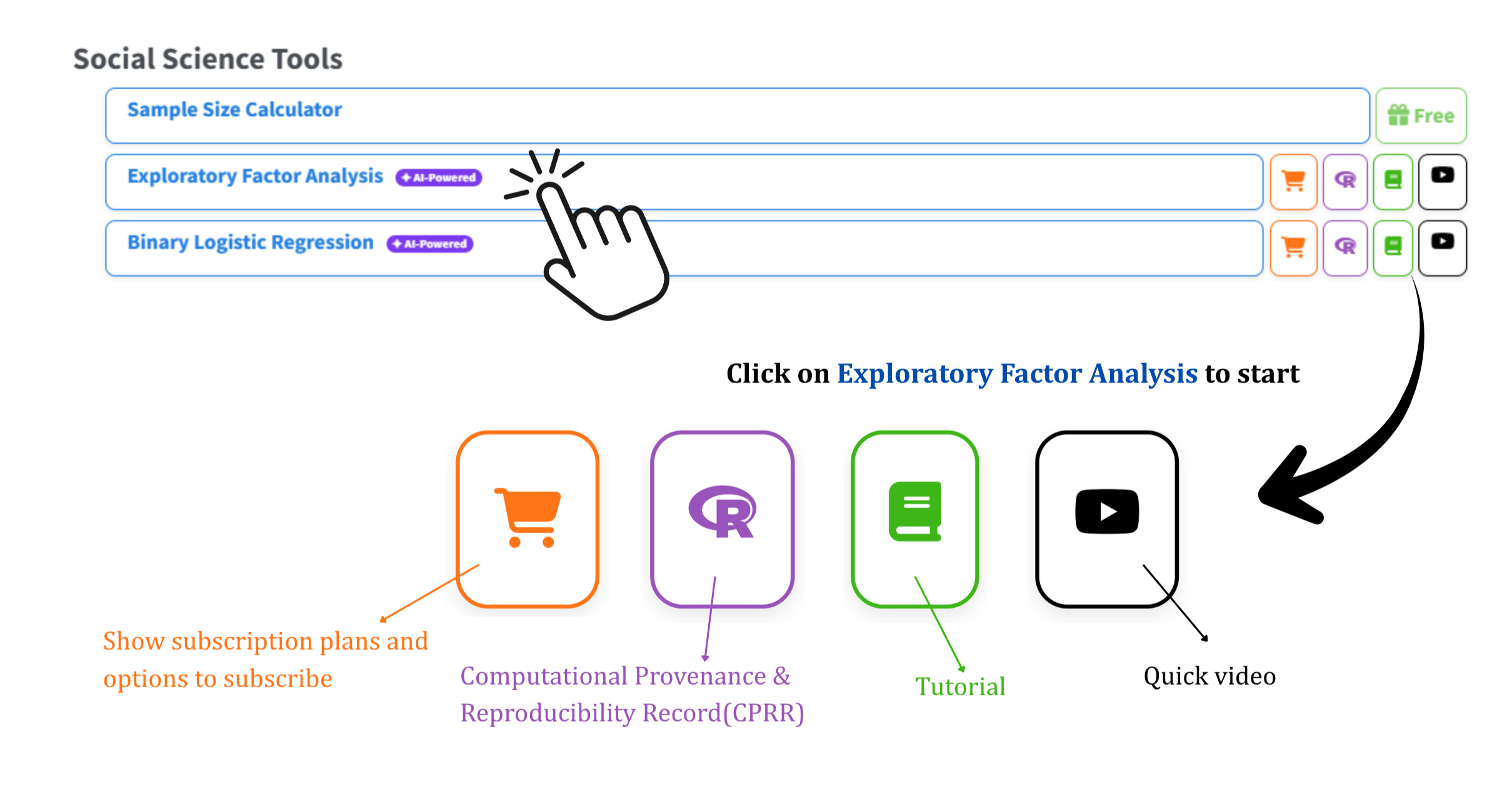
Open the RAISINS home page at www.raisins.live and go to the Social Science Tools section. Select the Exploratory Factor Analysis module (Figure 2).
No programming knowledge is required. You upload your data, select the variables, and RAISINS performs the complete analysis and produces publication-ready output.
3.1 Computational Provenance & Reproducibility Record
CPRR (Computational Provenance & Reproducibility Record) provides a transparent and comprehensive record. Click on the icon shown in Figure 2 to access CPRR and know about the computational workflow performed during the analysis. The record for this module states the R version and the exact version of every package used, names the specific function behind each reported result. CPRR lists every default parameter and decision rule applied by the module and provides fully runnable R code that reproduces each analytical step. Users can execute the code in R to independently reproduce and verify the results. It carries its own DOI.
For this module the record covers the complete chain: psych::KMO() and psych::cortest.bartlett() for data suitability, psych::fa.parallel() and psych::VSS() for determining the number of factors, psych::fa() for extraction and rotation, psych::alpha() for reliability, and how the variance explained, factor correlations, fit statistics and factor scores are obtained. The code runs on the bfi dataset supplied with the psych package, so every step can be executed without any RAISINS file.
To cite the platform itself in a paper, thesis, or report, use the RAISINS citation, available in APA, Harvard, and BibTeX formats at www.raisins.live/citation.html. That is the primary reference, and for most manuscripts it is all you need.
For the CPRR for the exploratory factor analysis module Click here.
Cite the RAISINS paper as your primary reference for the platform. Add the CPRR as supporting documentation when a journal asks for details of the computing environment, or when you want your methods section to be precise about versions and functions rather than saying “analysis was carried out using an online tool.” The CPRR supports the citation and ensures computational reproducibility.
4 Preview Mode and Quick Tour
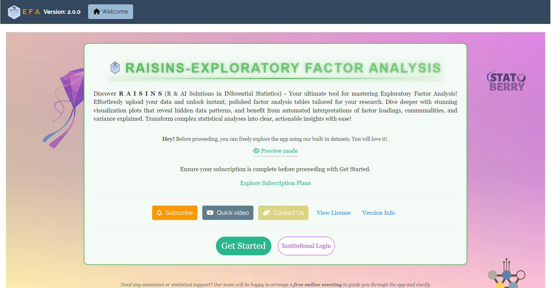
You can explore the entire module before subscribing by using Preview mode on the Welcome page. It loads built-in datasets, so you can try every feature, including the analysis, the plots, and the interpretation, without uploading your own data.
First-time users are also offered a Quick Tour. This is an interactive, step-by-step walkthrough that highlights each tab and control and explains what it does. You can replay it at any time from the Quick Tour tab in the top navigation.
5 The Example Dataset
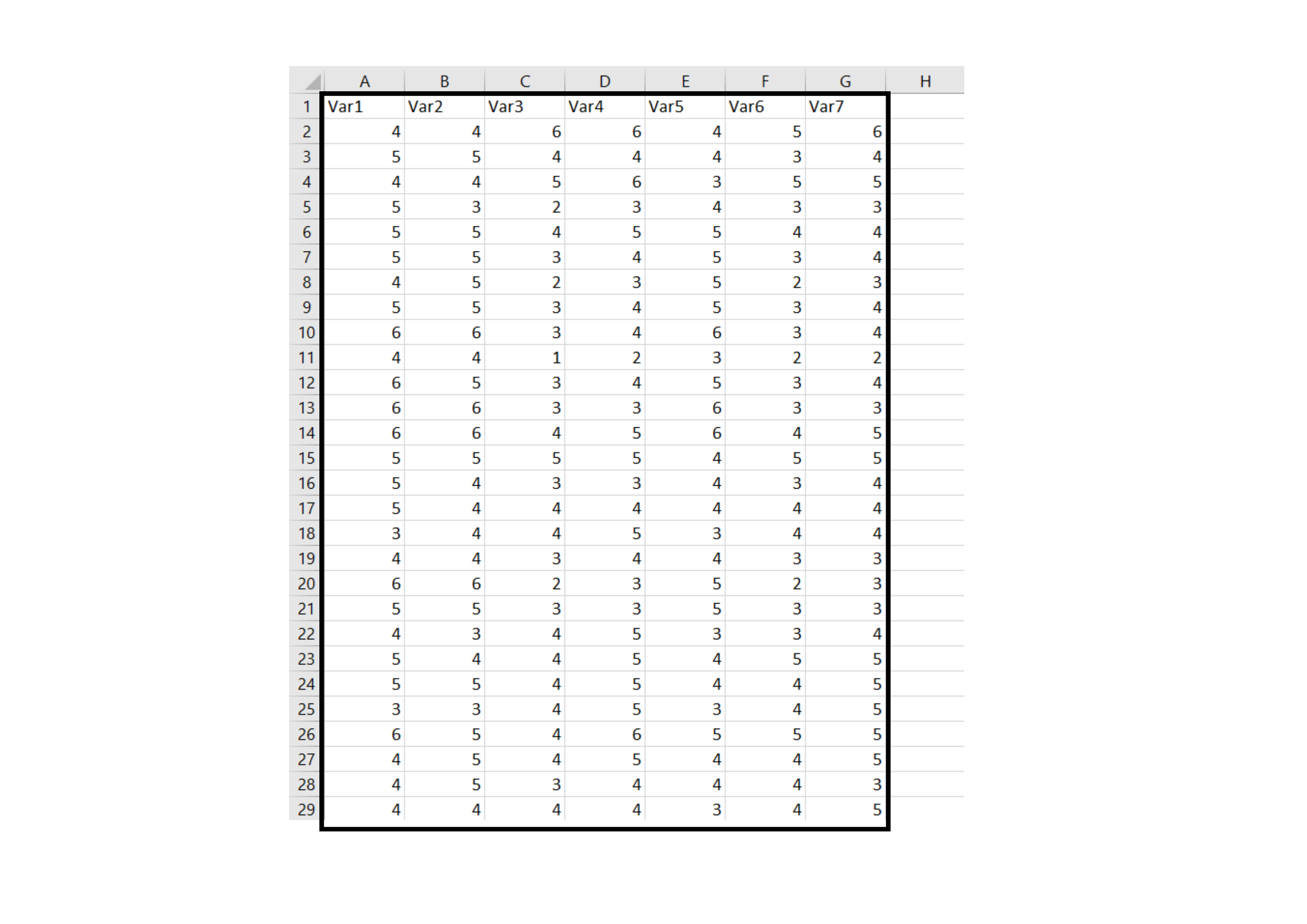
This tutorial uses Dataset 1, which is supplied with the module and can be downloaded from the Datasets tab. It contains 100 responses from a mobile app usability study. Each row is one farmer’s response, and each column is one of seven usability attributes, recorded as Var1 to Var7.
Unlike regression, factor analysis has no dependent variable. All seven variables enter the analysis on an equal footing, and every column selected must be numeric.
The objective is to find out whether the seven attributes represent seven distinct aspects of usability, or a smaller number of underlying dimensions. The data layout is shown in Figure 4.
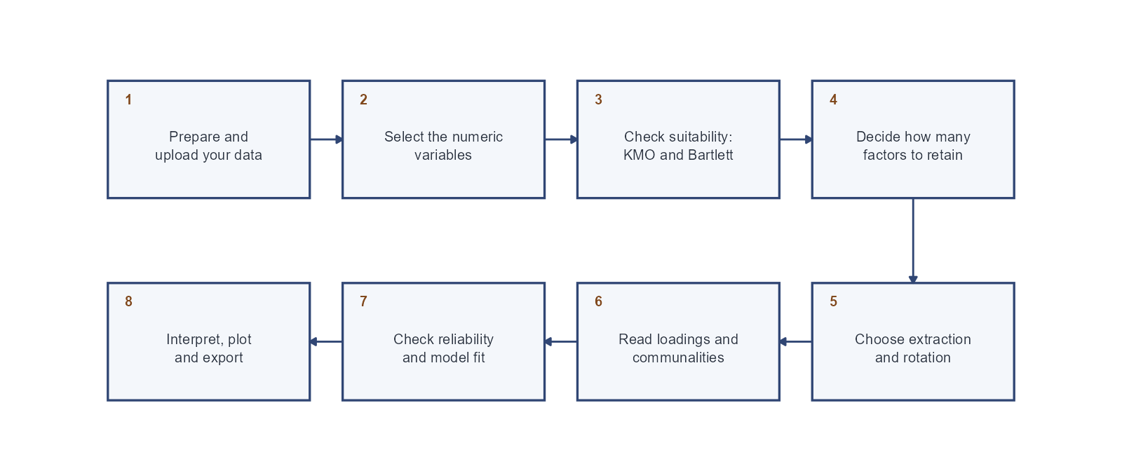
- Prepare your dataset.
- Upload the data and select the numeric variables.
- Check that the data are suitable using KMO and Bartlett’s test.
- Decide how many factors to retain.
- Choose an extraction method and a rotation.
- Read the loadings and communalities.
- Check the reliability of each factor and the model fit.
- Interpret the result, examine the plots, and export the tables and figures.
The sections below walk through each of these steps in detail.
6 Preparing Your Data
The quality of your analysis depends on the quality of your data. The required layout is simple: one row per observation, one column per variable, and all analysis columns numeric.
RAISINS provides four ways to prepare a correctly formatted dataset:
- Create it in MS Excel.
- Build it inside the app using Create Data.
- Download a built-in Model dataset and use it as a reference.
- Generate it through the RA-One chat assistant.
A commonly cited guideline suggests 5 to 10 observations per variable, with a practical floor of about 100 observations in total, though the sample size that is actually adequate depends less on this ratio and more on how strong the communalities are and how many variables define each factor (MacCallum, Widaman, Zhang, & Hong, 1999). The example dataset has 100 responses for 7 variables, a ratio of roughly 14:1, which is comfortably adequate by either standard. A small sample does not merely reduce precision; it can make the recovered factor structure itself unstable from one sample to the next. RAISINS reports this ratio for you in the Interpretation tab.
6.1 Preparing Data in MS Excel
Enter the variable names in the first row and one observation per row underneath, as shown in Figure 4. Leave no blank rows above the header, do not merge cells, and avoid trailing empty rows at the bottom of the sheet, which are a common cause of stray missing values.
Save the file as CSV (Comma delimited), or keep it as .xlsx. RAISINS reads both, but CSV is lighter and is recommended.
Always start column names with a letter. Use only letters, numbers, dots (.) or underscores (_). Avoid spaces and special characters.
6.2 Creating Data Inside RAISINS
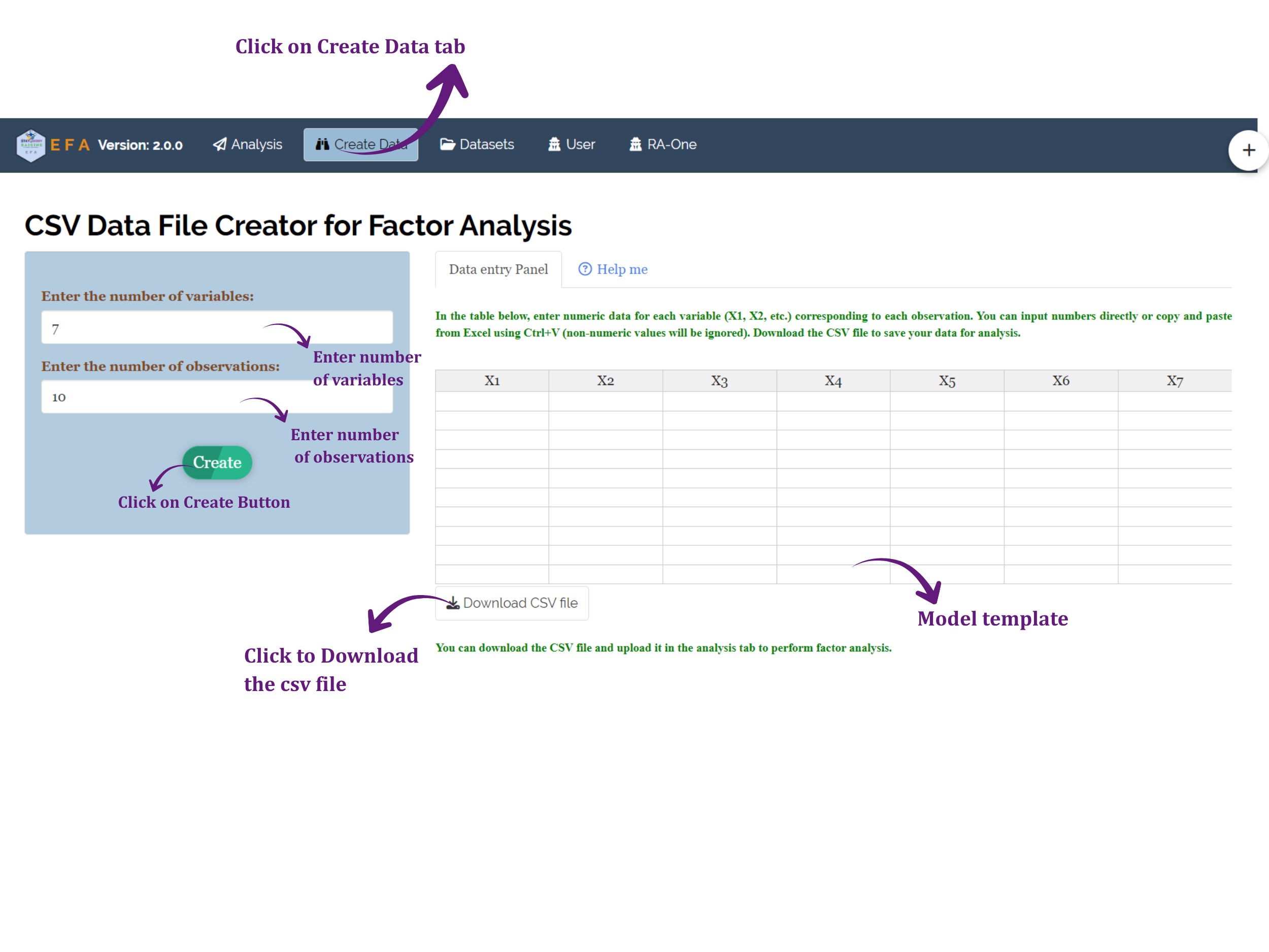
If you prefer not to use a spreadsheet, the Create Data tab builds the file for you. Enter the number of variables and the number of observations, then click Create. An editable grid appears in which you can type values directly or paste a block from Excel using Ctrl+V. Download the finished CSV and upload it in the Analysis tab.
6.3 Downloading Model Datasets
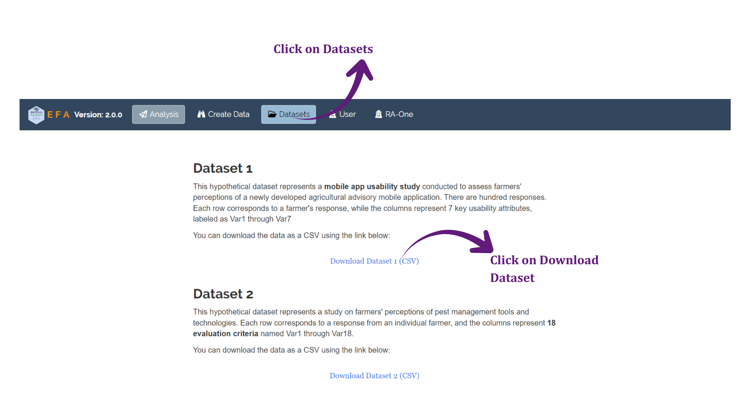
The Datasets tab holds two built-in example files. Dataset 1 is the mobile app usability study used throughout this tutorial, with 100 responses and 7 variables. Dataset 2 is larger, with 250 responses and 18 variables, and is useful for seeing how a multi-factor solution behaves. Download either one to inspect the expected layout.
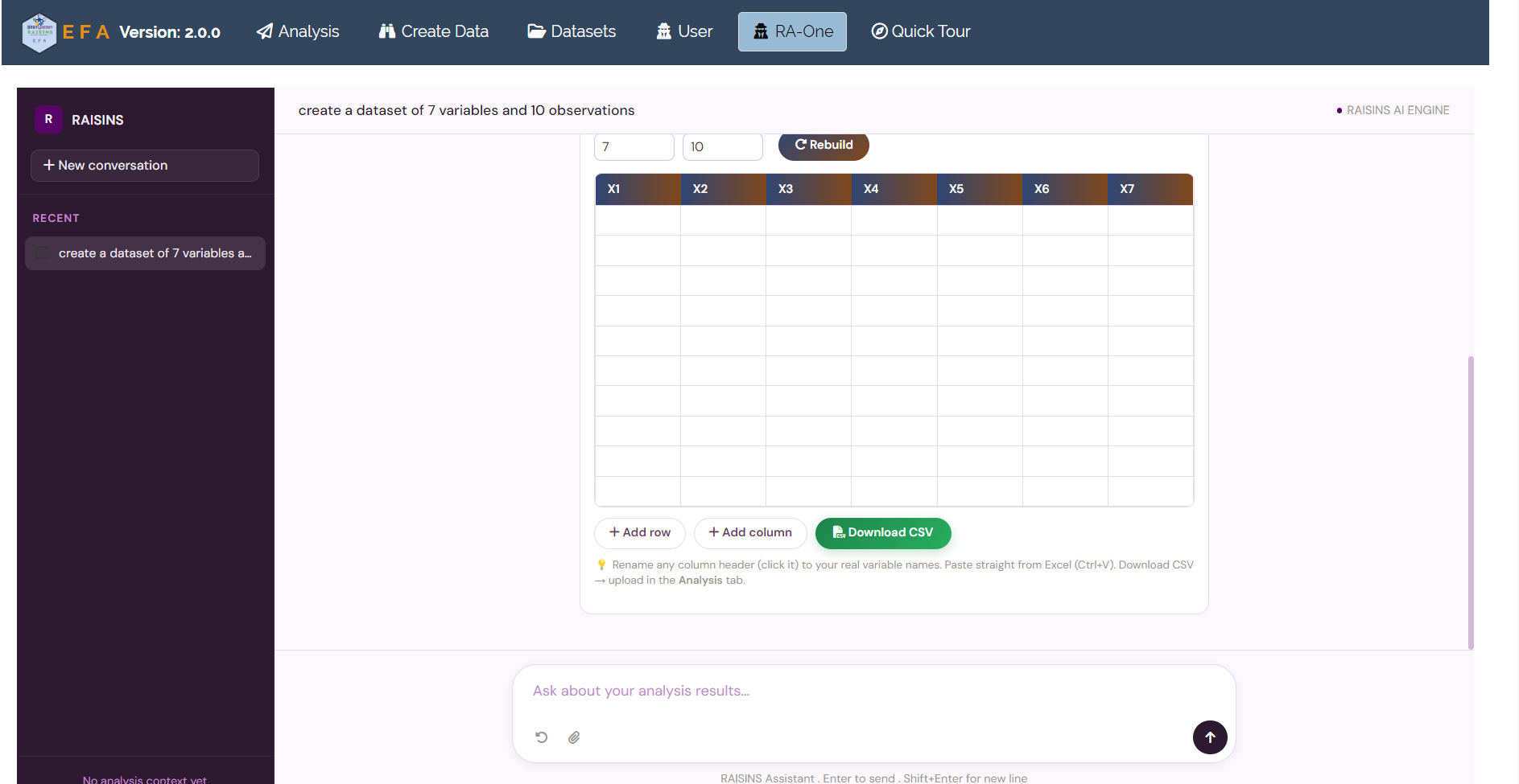
6.4 Creating a Dataset Using RA-One
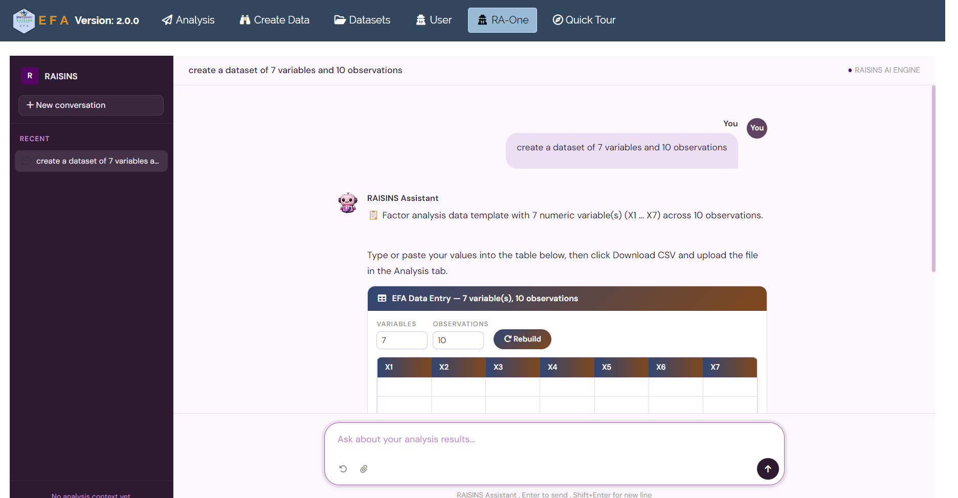
Open the RA-One tab, or click the floating assistant button in the corner of the screen, and describe what you need in plain language:
“Create a factor analysis dataset with 7 variables and 100 observations”
RA-One builds an editable data-entry table inside the chat, with Add row and Add column buttons and a Download CSV button. Values can be pasted from Excel or entered directly. If you mention only the number of variables, RA-One will ask how many observations you want before building the table.
7 The Analysis Tab
Before a file is uploaded, the Analysis tab shows four help icons covering data upload, how to perform the analysis, choosing the number of factors, and extraction and rotation methods. Each opens a short guide.
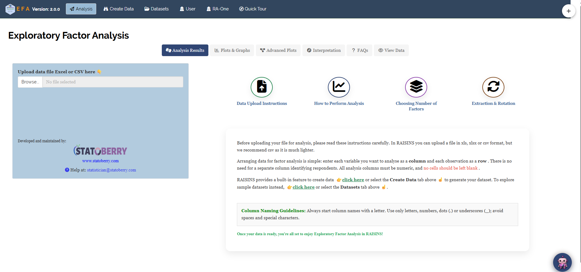
Upload your file using Browse in the sidebar. A variable selector appears; tick the numeric columns to be analysed, which for the example dataset is all seven. Then click Run Analysis.
A settings panel appears above the results with four controls (Figure 10).
- Number of Factors - Pre-filled with the number suggested by parallel analysis, and adjustable.
- Extraction Method - How the factors are obtained from the correlation matrix. Principal Axis is the default and makes no distributional assumptions. Maximum Likelihood provides formal fit statistics and assumes approximate normality. Minimum Residual, Weighted Least Square, Generalized Least Square, Minimum Chi-Square and Alpha Factoring are also available.
- Type of Rotation - The eight options described in Section 2.
- Digits after decimal - The number of decimal places shown in every results table, from 1 to 5, with a default of 3. This is a display setting only. It never changes the computation, and it applies to the downloadable report as well.
In practice the different extraction methods usually produce very similar loadings on well-behaved data, so this choice matters less than the choice of rotation. Maximum Likelihood is preferable when a formal chi-square test of fit is needed and the variables are approximately multivariate normal; Principal Axis is a robust default that avoids this assumption.
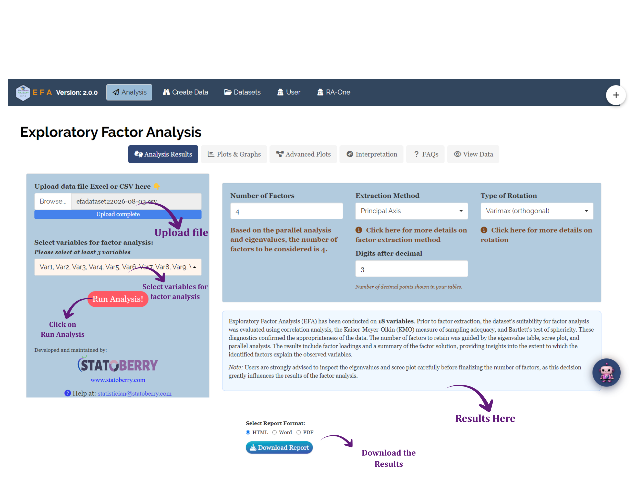
Number of factors: 2 · Extraction: Principal Axis · Rotation: Varimax · Digits: 3
Apply these to Dataset 1 and every number reported below will match exactly.
8 Analysis Results
The Analysis Results sub-tab presents the tables in the order they should be read: first whether the data are suitable for factor analysis, then how much variance the factors explain, then what the factors mean, and finally how well the model fits.
8.1 Table 1: KMO and Sampling Adequacy
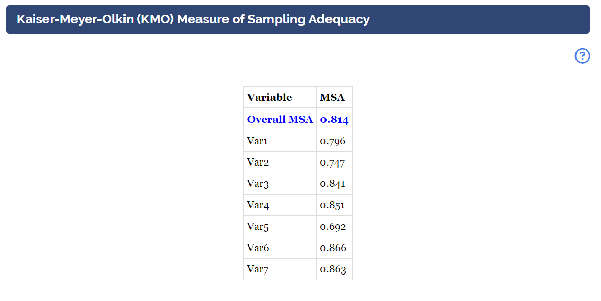
The Kaiser-Meyer-Olkin (KMO) measure compares the size of the ordinary correlations with the size of the partial correlations. When variables genuinely share underlying factors, their correlations remain large after the influence of the other variables is removed, and KMO approaches 1. When each correlation is isolated, KMO falls towards 0. This is checked before extraction because a low value means there is not enough shared variance for factoring to recover anything meaningful, whatever the subsequent tables might suggest.
The table reports an Overall MSA and an individual MSA for every variable.
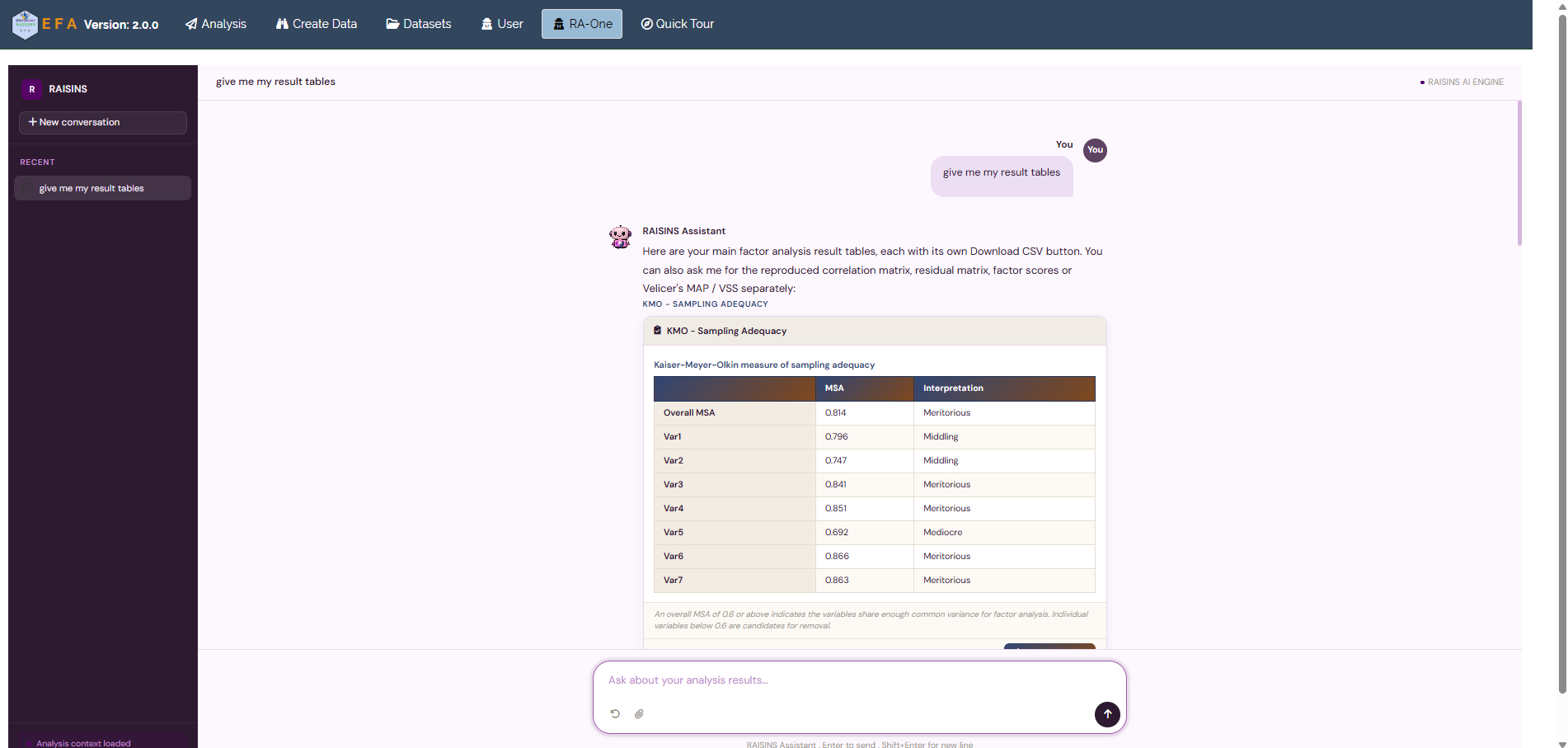
In the example, the overall MSA is 0.814, which is meritorious. Every individual variable also exceeds 0.6, ranging from 0.692 for Var5 to 0.866 for Var6. No variable needs to be removed on this criterion.
Interpreting KMO values
Kaiser’s original labels, still widely used as an informal guide rather than a strict statistical rule, are:
| KMO value | Interpretation |
|---|---|
| 0.90 and above | Superb |
| 0.80 to 0.89 | Meritorious |
| 0.70 to 0.79 | Middling |
| 0.60 to 0.69 | Mediocre |
| Below 0.60 | Unacceptable; factor analysis is not advisable |
The overall value decides whether to proceed. The per-variable values are diagnostic: a single variable well below 0.6 while the others are healthy is a candidate for removal, because it does not share variance with the rest.
8.2 Table 2: Bartlett’s Test of Sphericity
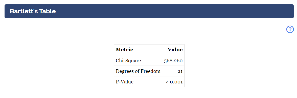
Bartlett’s test examines the same question from the opposite direction. Its null hypothesis is that the correlation matrix is an identity matrix, in which every variable is uncorrelated with every other. If that were true, there would be no shared structure to extract. A significant result is therefore required before proceeding.
In the example, Bartlett’s test gives a chi-square of 568.260 on 21 degrees of freedom, with p < 0.001. The null hypothesis is rejected, confirming that sufficient correlations exist among the seven variables.
Bartlett’s test is sensitive to sample size and becomes significant almost automatically in large datasets. Treat it as a minimum requirement rather than strong evidence, and rely on the KMO value for the more informative judgement. A non-significant result, on the other hand, is informative in its own right: it indicates that the variables do not share enough correlation for factor analysis to be meaningful, regardless of sample size.
8.3 Table 3: Eigenvalues and Variance Explained
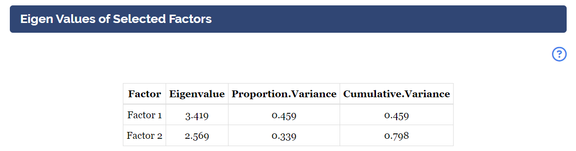
This table reports, for each retained factor, its eigenvalue, the proportion of total variance it explains, and the cumulative total.
In the example, the two retained factors have eigenvalues of 3.419 and 2.569. The first explains 46.0% of the total variance and the second a further 33.8%, giving a cumulative 79.8%.
The complete set of eigenvalues is 3.419, 2.569, 0.268, 0.224, 0.207, 0.170 and 0.143. Only the first two exceed 1, and the third is far below it. The two-factor solution is therefore strongly supported, and this pattern is examined more formally in Section 9.
In the physical sciences 80% to 90% may be expected. In social science and questionnaire research, 50% to 60% is often considered acceptable. The 79.8% obtained here is strong by any standard.
8.4 Table 4: Factor Loadings, Communalities and Uniqueness
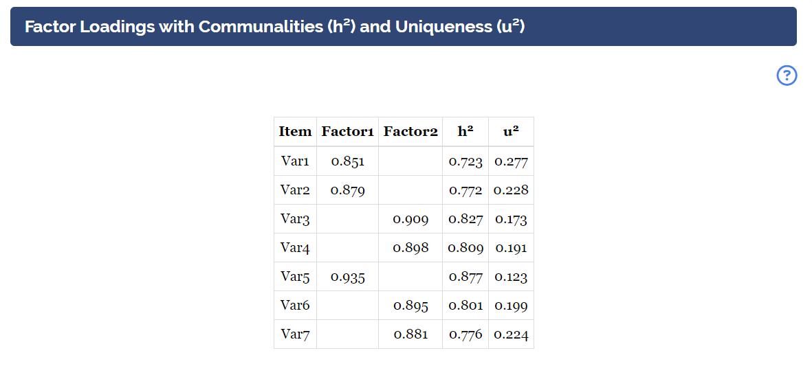
This is the central table of the analysis. Each row is a variable, each factor column holds that variable’s loading, and the final two columns report the communality and the uniqueness.
In the example, the structure is unusually clear.
- Factor 1 is defined by Var5 (0.935), Var2 (0.879) and Var1 (0.851).
- Factor 2 is defined by Var3 (0.909), Var4 (0.898), Var6 (0.895) and Var7 (0.881).
Every one of these loadings exceeds 0.85 on its own factor, and the corresponding loadings on the other factor lie between −0.069 and 0.038. There is not a single cross-loading in the table, which is what is meant by simple structure. Communalities range from 0.723 for Var1 to 0.877 for Var5, so the two factors explain between 72% and 88% of the variance of every variable.
The seven usability attributes therefore represent two underlying dimensions rather than seven separate ones. Naming those dimensions is the researcher’s task, not the software’s: a factor is named from what its defining items have in common, read against their actual wording and the subject-matter context, not from the arbitrary order in which the software lists them. Because Var1 to Var7 are anonymised placeholders in this dataset, this tutorial does not assign names to the two factors here; with real questionnaire items, this step is where the substantive interpretation of the analysis begins.
Understanding the loadings table
| Column | Meaning |
|---|---|
| Factor 1, Factor 2, … | The loading of that variable on each factor. Values of 0.4 or above in absolute value are considered meaningful |
| h² (communality) | The proportion of that variable’s variance explained by all retained factors together |
| u² (uniqueness) | The remaining proportion, equal to 1 − h², specific to that variable or due to measurement error |
Read down one factor column at a time and note which variables load at 0.4 or above; those variables define that factor. Then scan the h² column for values below 0.3, which indicate variables the solution does not explain. Finally check for variables loading above 0.4 on more than one factor; a cross-loading is often the first sign that a different number of factors, or a different rotation, should be examined.
8.5 Table 5: Reliability of Each Factor
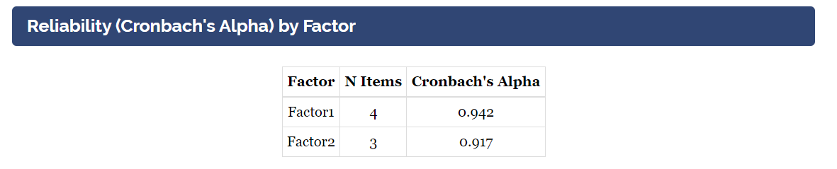
Once a group of variables has been identified as belonging to a factor, the next question is whether they are consistent enough to be combined into a single score. Cronbach’s alpha measures this internal consistency. RAISINS computes it for each factor using the variables whose dominant loading falls on that factor.
In the example, Factor 1 has an alpha of 0.942 across its four variables and Factor 2 an alpha of 0.917 across its three. Both are excellent, so either group could be averaged into a single summary score.
Interpreting Cronbach's alpha
These bands are a commonly used guideline rather than a strict rule:
| Alpha | Interpretation |
|---|---|
| 0.90 and above | Excellent |
| 0.80 to 0.89 | Good |
| 0.70 to 0.79 | Acceptable |
| 0.60 to 0.69 | Questionable |
| Below 0.60 | Poor |
Alpha increases as items are added, so a high value on a long scale is less impressive than the same value on a short one. A factor with fewer than two variables has no alpha, and RAISINS reports this rather than producing a value. When alpha for a factor is low, check whether the factor is defined by only two items, or whether one item loads noticeably more weakly than the others; removing that item and repeating the analysis often improves consistency.
A high alpha shows that a set of items behaves consistently; it does not, on its own, show that the items measure what the researcher intends, and it does not prove that the set is unidimensional. Report reliability alongside the factor structure, not as a substitute for it.
8.6 Table 6: Factor Correlation Matrix
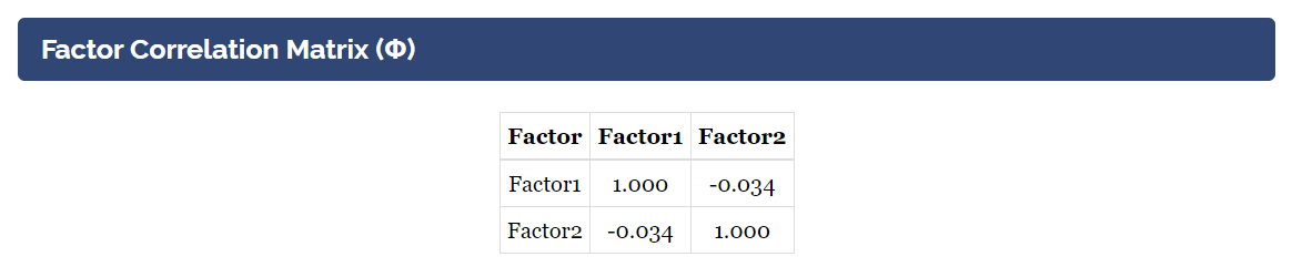
This table appears only when an oblique rotation has been selected and two or more factors are extracted, because only an oblique rotation permits the factors to correlate.
It answers a practical question: were the factors genuinely independent? If the off-diagonal values are close to zero, an orthogonal rotation such as Varimax would produce essentially the same solution. If they are substantial, the underlying constructs overlap, which is itself a finding.
Because this tutorial uses Varimax throughout, this table is not produced for the primary analysis. Repeating Dataset 1 with Oblimin illustrates it directly (Figure 16): the two factors correlate at only −0.034, close enough to zero that the orthogonal Varimax solution used in this tutorial loses essentially nothing by holding the factors uncorrelated. Fitting an oblique rotation once as a check, even when an orthogonal rotation is your final choice, is a reasonable way to confirm that assumption rather than take it for granted.
8.7 Table 7: Model Fit
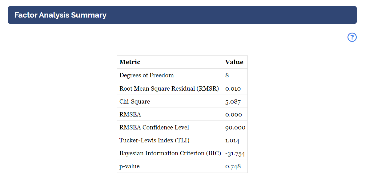
The final table reports how well the retained factors reproduce the original correlation matrix.
In the example, with 8 degrees of freedom, RMSR = 0.010 and RMSEA = 0.000 (90% confidence interval 0.000 to 0.084), and TLI = 1.014. The chi-square is 5.087 with p = 0.748, which is not significant, so the hypothesis of perfect fit cannot be rejected. BIC = −31.754. The two-factor model reproduces the observed correlations almost exactly.
The RMSEA point estimate of 0.000 should be read together with its confidence interval, 0.000 to 0.084. In a sample of 100 this interval is fairly wide, and it shows that the data remain consistent with somewhat weaker fit than the point estimate alone would suggest. This is a normal consequence of a modest sample size rather than a defect in the model.
Understanding the fit statistics
The following bands, drawn from the structural equation modelling literature, are common practical guidelines rather than strict pass or fail thresholds:
| Statistic | Meaning and guideline |
|---|---|
| RMSR | Root mean square residual, the average size of the correlations the model fails to reproduce. 0.08 or below indicates good fit |
| RMSEA | Penalises model complexity. 0.06 or below indicates close fit; above 0.10 indicates poor fit |
| TLI | Compares the model with one having no factors. Values approaching 0.95 or higher indicate good fit |
| Chi-square and p-value | Tests the hypothesis of perfect fit. Here a non-significant result is desirable |
| BIC | Used only for comparing competing models, where a lower value is preferred |
TLI can exceed 1 and RMSEA can equal 0 when a model fits better than its degrees of freedom would predict. These are not errors; they indicate fit at or beyond the ceiling the index can express. The chi-square test is also sensitive to sample size: it can reject trivially small misfit in a large sample, and fail to detect real misfit in a small one.
8.8 Further Tables
Below the main results RAISINS also reports the reproduced correlation matrix, which contains the correlations implied by the factor solution; the residual matrix, which is the observed matrix minus the reproduced one, where off-diagonal values above roughly |0.05| identify variable pairs the model handles poorly; and the correlation matrix of the original variables with significance stars.
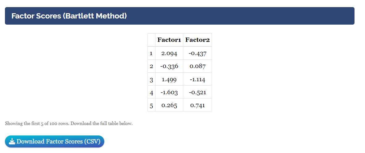
The factor scores table gives each respondent’s estimated standing on each factor, computed by the Bartlett method. A preview is shown on screen and the complete table can be downloaded as a CSV file. Factor scores are what you need when the factors are to be used as variables in a later regression, clustering or analysis of variance; bear in mind that they are estimates rather than directly observed values, and different estimation methods give slightly different scores.
9 Deciding How Many Factors to Retain
The number of factors is the single most consequential decision in an exploratory factor analysis, and no criterion settles it alone. RAISINS reports four, and they should be read together.
9.1 Kaiser’s Criterion
Retain every factor with an eigenvalue greater than 1, on the reasoning that such a factor explains more variance than one original variable. This rule is simple but is known to overestimate the number of factors, so it should not be used by itself.
In the example, exactly two eigenvalues exceed 1.
9.2 The Scree Plot
The scree plot shows the eigenvalues in descending order. The point at which the curve stops falling steeply and flattens is called the elbow. Factors before the elbow are retained.
In the example, the curve falls from 3.419 to 2.569 and then drops sharply to 0.268, producing an unmistakable elbow after the second factor. The elbow is not always this obvious; when the descent is gradual, this criterion is a matter of judgement and the other three should carry more weight.
9.3 Parallel Analysis
Parallel analysis compares your eigenvalues with those obtained from randomly generated data of the same size. A factor is retained only if its real eigenvalue exceeds the corresponding random one. This is generally regarded as the most reliable of the criteria, and RAISINS uses it to pre-fill the Number of Factors control.
In the example, parallel analysis suggests 2 factors.
9.4 Velicer’s MAP and Very Simple Structure
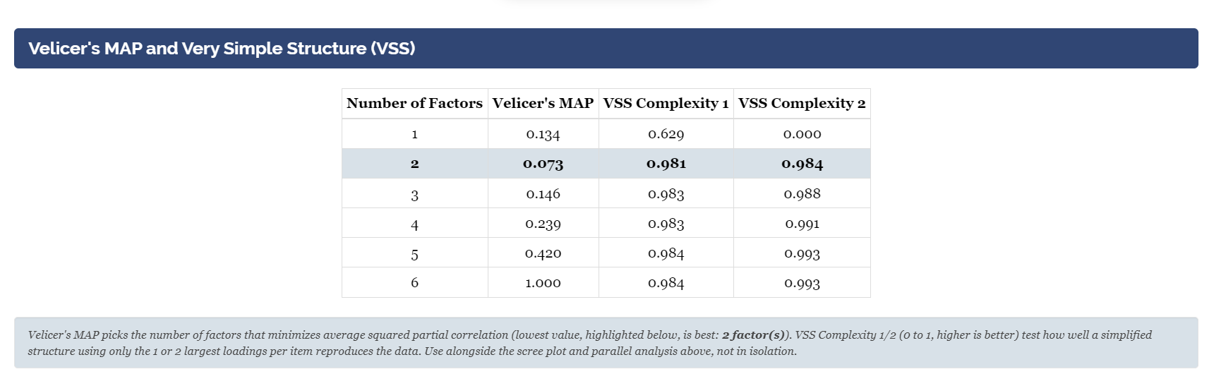
Displayed beneath the parallel analysis plot, this table reports two further criteria. Velicer’s MAP removes the influence of successive factors and monitors the average squared partial correlation; the number of factors that minimises the MAP value is the recommendation, and RAISINS highlights that row. VSS Complexity 1 and 2 assess how well a deliberately simplified version of the solution, retaining only the largest one or two loadings per variable, reproduces the data. Higher values are better.
In the example, the MAP values are 0.134, 0.073, 0.146, 0.239, 0.420 and 1.000, reaching their minimum at 2 factors.
All four criteria agree on two factors in this example, which is the ideal case and is not guaranteed in real data. When the criteria disagree, a defensible approach is to fit each competing solution in turn and compare them on interpretability: does the pattern of loadings produce factors that make substantive sense given what the variables actually measure, and does the theoretical or research context favour one solution over another? Statistical criteria narrow the range of plausible solutions; they do not remove the need for judgement, and the reasoning behind the final choice should be reported alongside the result.
10 Plots and Graphs
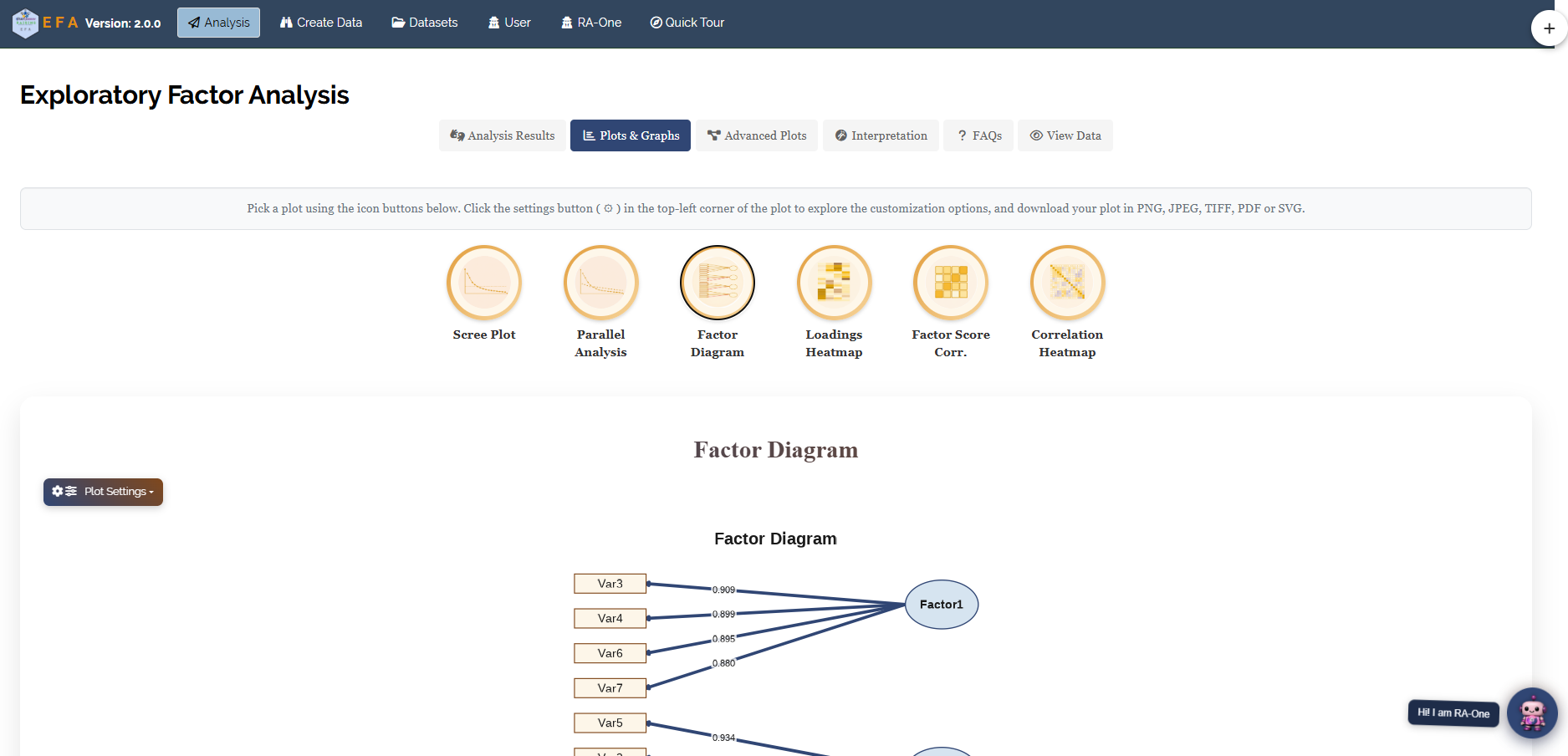
The Plots & Graphs sub-tab presents six figures behind a row of icon buttons. Selecting an icon displays the corresponding plot, and the active icon is highlighted. Each plot has its own settings panel controlling titles, labels, colours, themes and plot-specific options, and each can be downloaded as PNG, JPEG, TIFF, PDF or SVG at a chosen width, height and resolution.
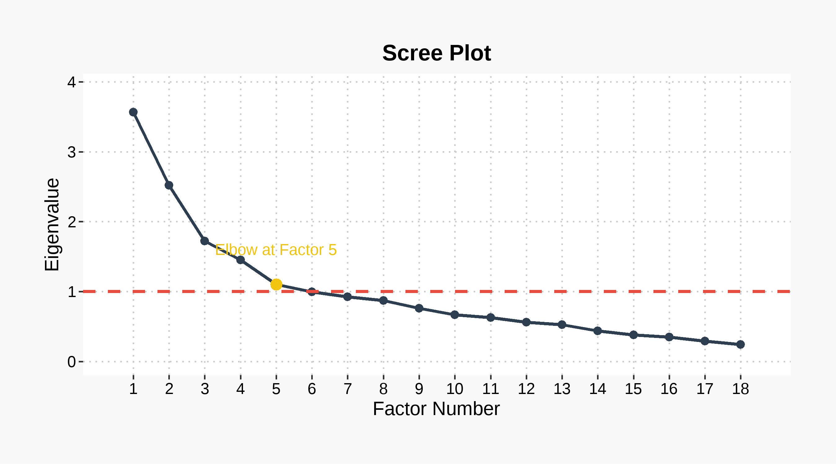
Scree plot, the eigenvalues of all possible factors in descending order. The elbow, where the curve flattens, marks the point beyond which additional factors contribute little.
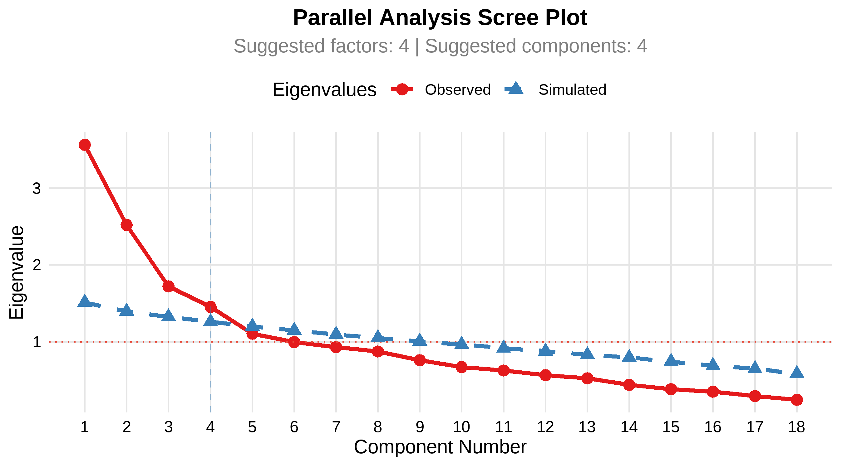
Parallel analysis, your eigenvalues plotted against those from randomly simulated data of the same size. Retain the factors whose real eigenvalue exceeds the simulated one.
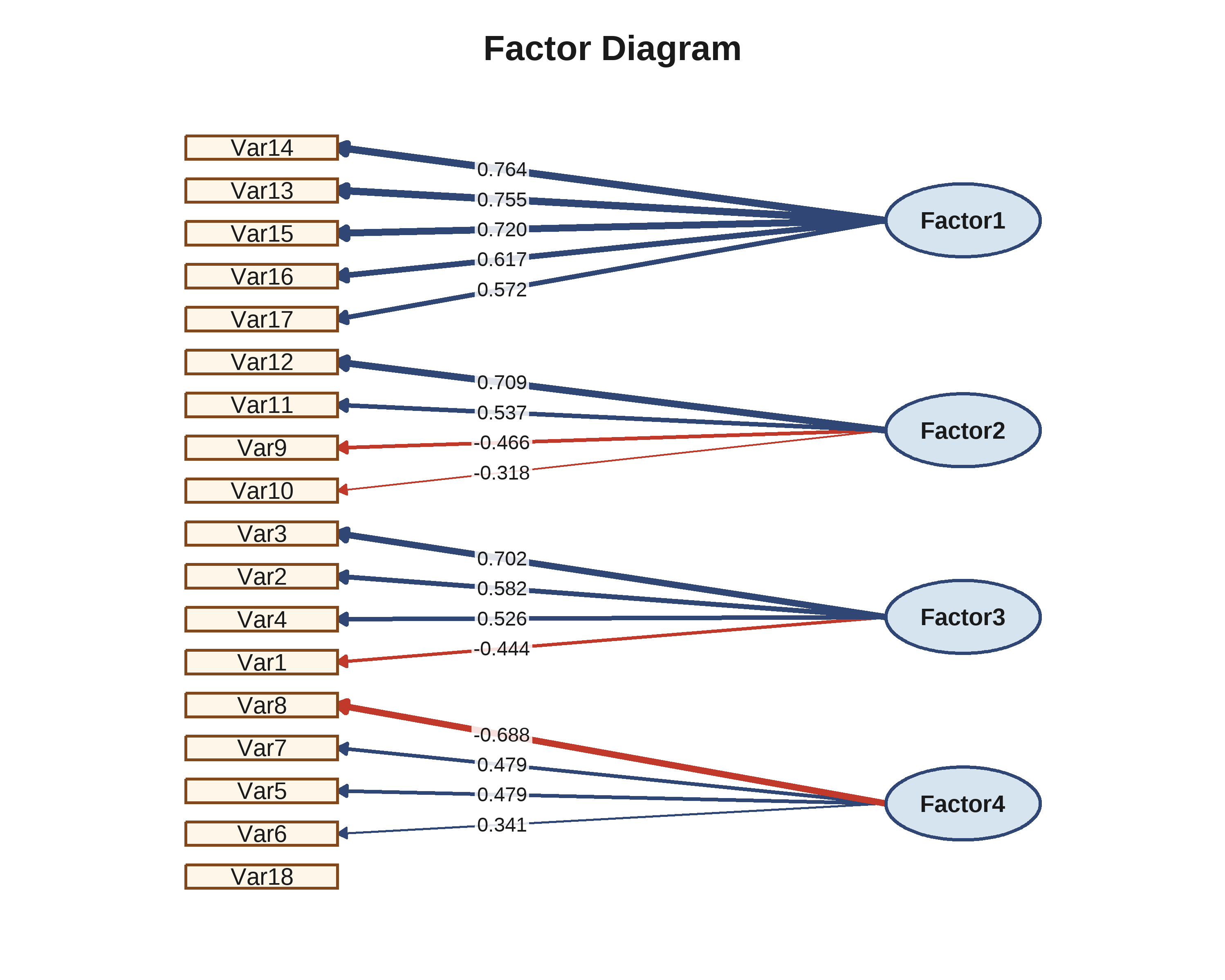
Factor diagram, a path diagram drawing an arrow from each factor to the variables it explains, labelled with the loading. Line thickness reflects loading strength.
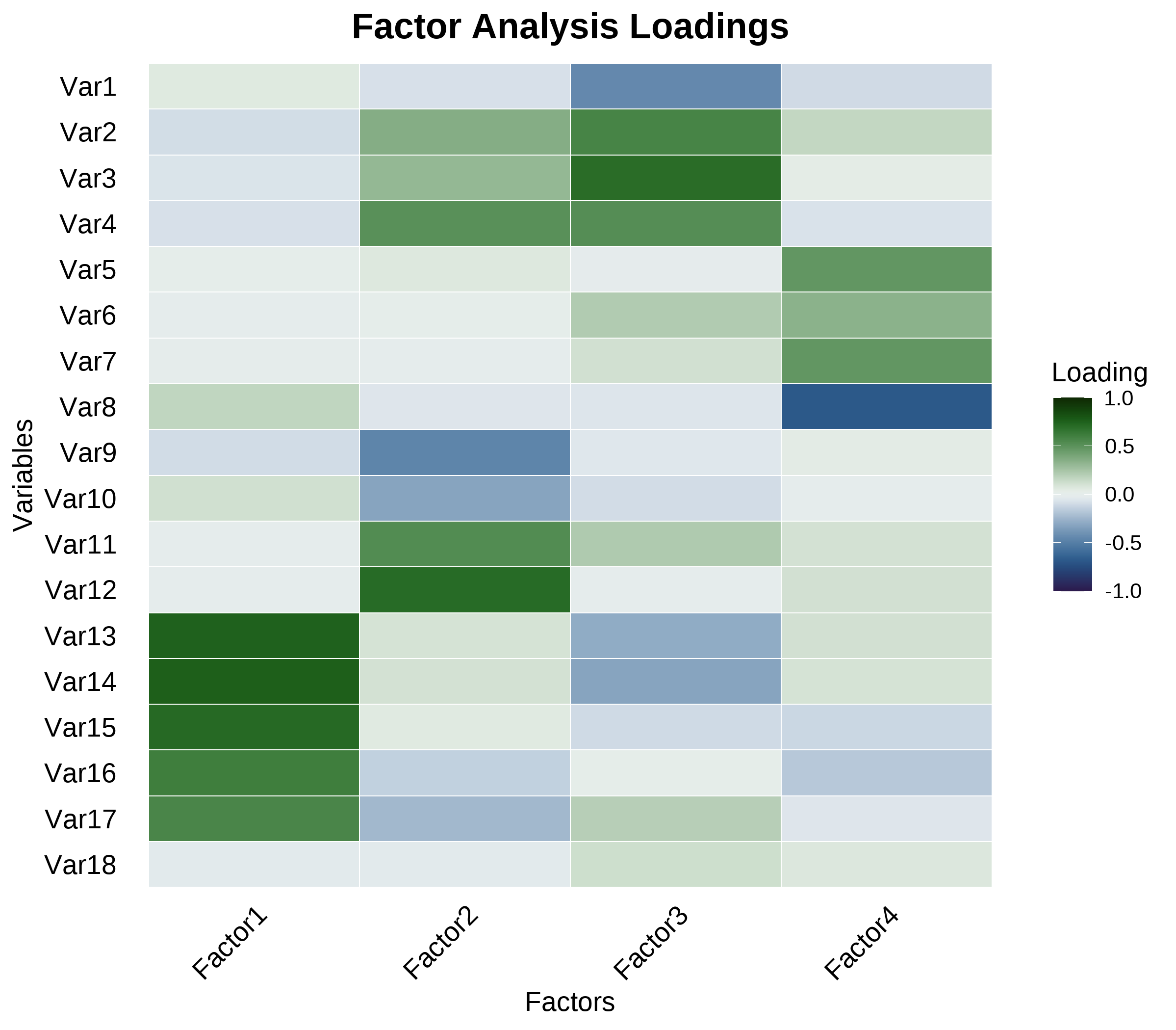
Loadings heatmap, the complete loadings table rendered as colour. Simple structure appears as a clean blocky pattern of strong and near-zero cells.
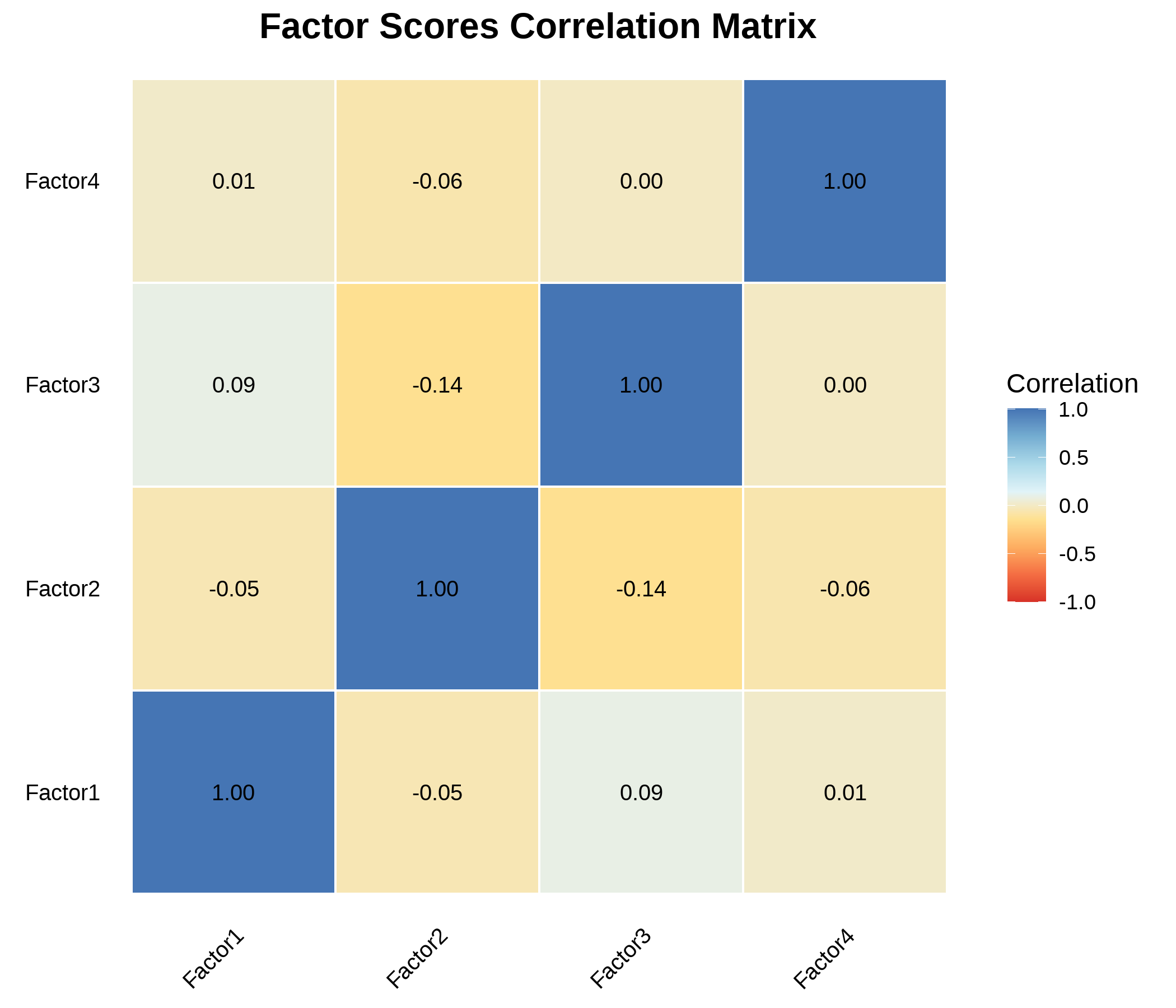
Factor scores correlation, the correlations among the computed factor scores. Under an orthogonal rotation these are near zero off the diagonal.
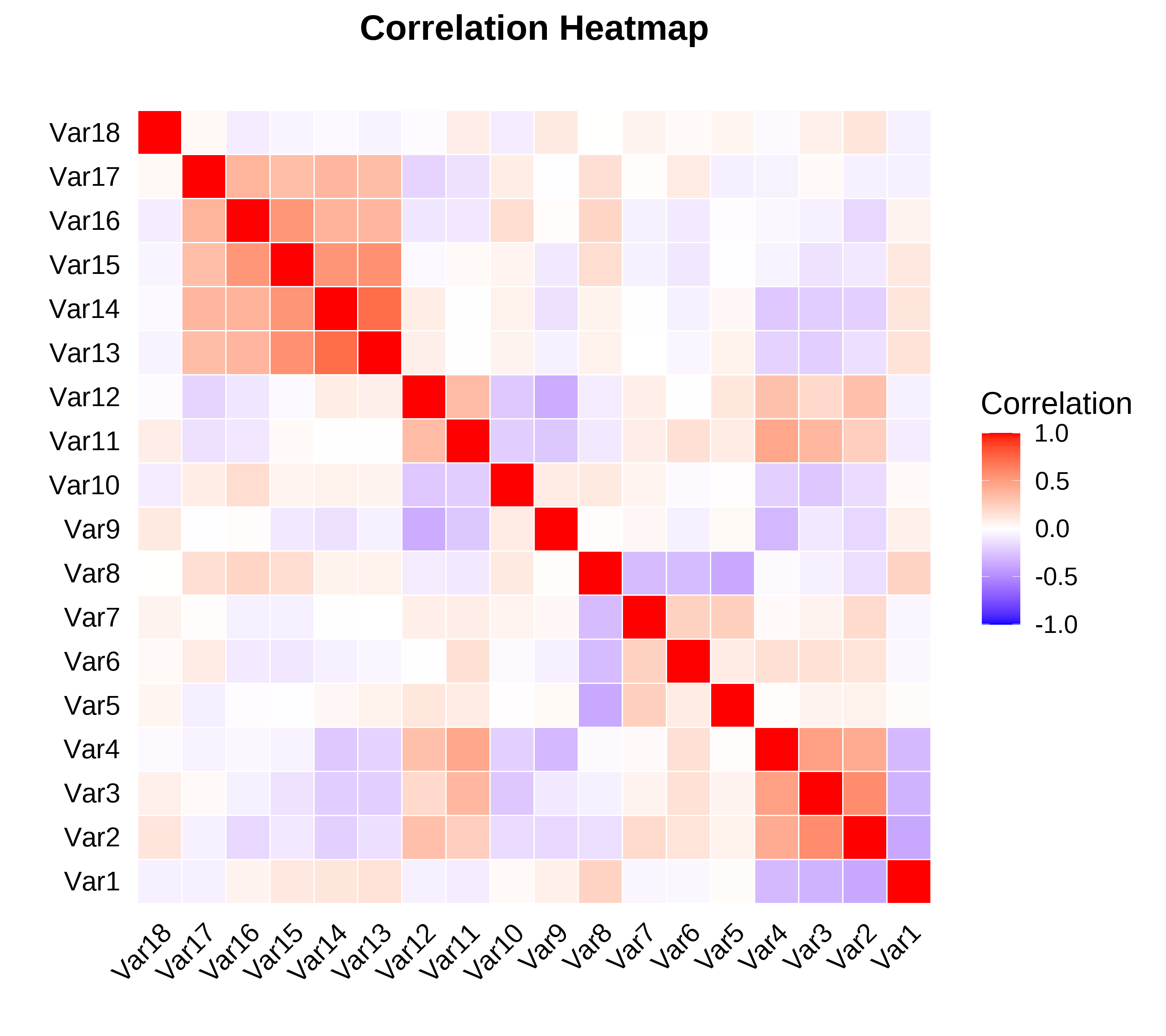
Correlation heatmap, the correlations among the original variables before factoring. Blocks of strong colour are the visual signature of the factors about to be extracted.
In the example, the scree plot and the parallel analysis plot both point to two factors, and the factor diagram shows four arrows from Factor 1 to Var3, Var4, Var6 and Var7, three from Factor 2 to Var1, Var2 and Var5, and no crossing paths.
The factor diagram has its own controls for the minimum loading drawn as a path, whether to show only each variable’s dominant loading or every loading above the threshold, whether to display factor-correlation arcs for oblique solutions, and the colours of each element. Its height also increases automatically with the number of variables, so wide datasets remain readable.
11 Advanced Plots
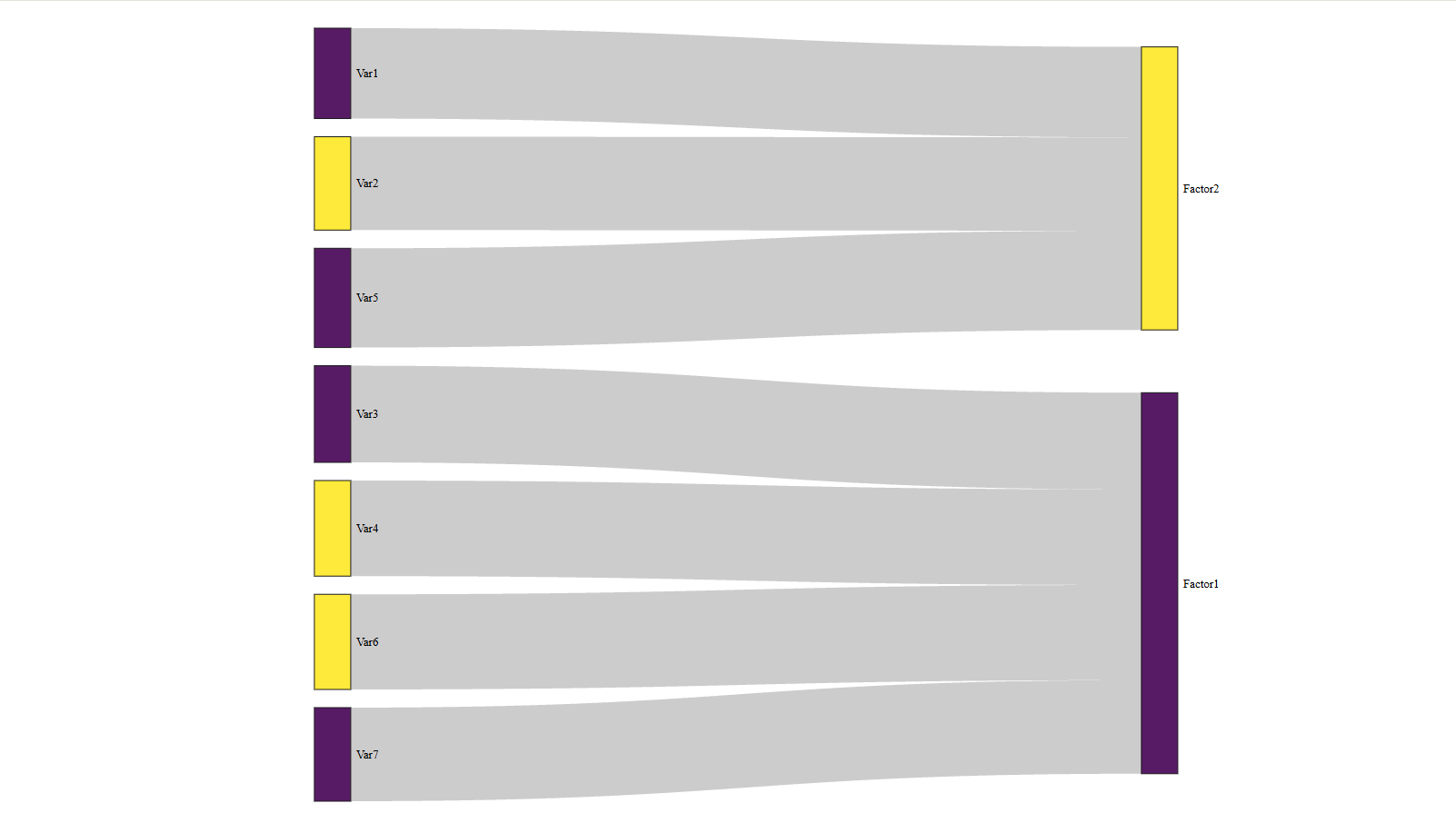
The Advanced Plots sub-tab contains a Sankey diagram of the loadings. It is an alternative to the factor diagram and is particularly effective when many variables load on several factors. Variables appear on one side and factors on the other, with the width of each ribbon reflecting the strength of the loading. The minimum loading threshold, node width and spacing, font size and colour palette are all adjustable.
12 Interpretation
The Interpretation sub-tab produces a written account of the analysis. Click Generate Interpretation and the text is typed out section by section: an overview of the settings used and whether the sample size was adequate, the suitability evidence, the factor solution and variance explained, the variables defining each factor with their communalities, the reliability of each factor, the factor correlations where applicable, the model fit with its thresholds, the strongest correlations among the variables, and a reference list.
Two buttons are provided. Stop ends the typing animation and displays the complete text immediately. Copy places the entire interpretation on the clipboard.
The text is generated from the same fitted model as the tables in the Analysis Results sub-tab, so the values quoted always agree with the values displayed. It also respects the Digits after decimal setting.
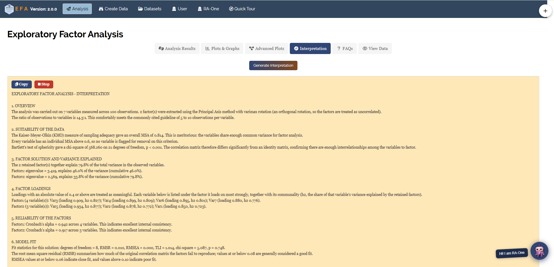
The automatic interpretation is a drafting aid. It reports what the statistics show, but it cannot know what your variables measure, whether your sample is representative, or whether a two-factor solution is theoretically sensible in your field. Review it and rewrite it in your own words before submission.
13 RA-One Chat Assistant
RA-One is the AI assistant built into the module, available from the RA-One tab or the floating button in the corner of the screen. It can read your fitted results, so questions can be asked about your own analysis rather than about factor analysis in general. It is best treated as a knowledgeable research assistant rather than a final authority: it retrieves and describes your fitted results accurately, but the scientific judgement, including what a factor should be called and whether a solution is theoretically defensible, remains the researcher’s.
It handles four kinds of request:
- Questions about your results - for example “Interpret my results”, “Which variables load on which factor?” or “Is my KMO acceptable?” Answers are drawn from your fitted model, and RA-One states plainly when a value is not available rather than estimating one.
- Result tables - asking for “result tables” returns the main tables, each with its own Download CSV button. Individual tables can be requested by name, such as “show the residual matrix” or “factor scores table”, and a single variable can be examined with “results for Var3”.
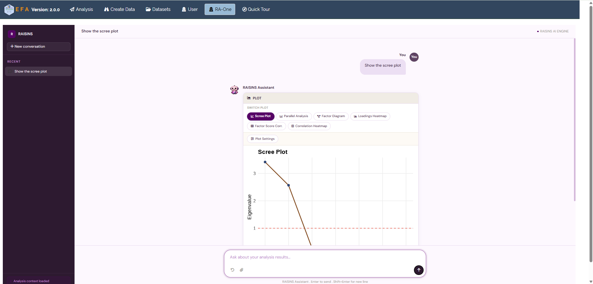
- Plots - naming a plot, such as “show the scree plot”, renders it inside the conversation with buttons to switch plot type and a panel to restyle it.
- Concepts and data preparation - for example “What is a communality?” or the dataset generation described in Section 6.4.
RA-One is powered by an external large language model. Your questions and a summary of your results are transmitted to that provider in order to generate answers. RAISINS does not store your data or your conversations, and everything is cleared when the session ends. The assistant is available on Institutional and Individual Full Licence plans.
14 Reporting EFA in a Manuscript
A completed analysis is useful to other researchers only if it is reported with enough detail to be judged, and where possible reproduced. Journals differ in exactly what they require, but the following is generally expected wherever exploratory factor analysis is reported: the sample and the variables analysed; the evidence considered for the suitability of the data; how the number of factors was decided, and which criteria were consulted; the extraction method and rotation used, with the reasoning behind the rotation choice; the number of factors retained and the variance they explain; the factor loadings, usually presented as a full table; communalities where they are informative; the reliability of each factor; model fit statistics where the extraction method supports them; and the interpretation and naming of the factors.
The paragraph below illustrates this using the Dataset 1 results reported throughout this tutorial. It is intended as an example of the level of detail expected, not as text to be copied into a manuscript without adaptation to the actual study, sample and variables.
The seven usability items were subjected to exploratory factor analysis using principal axis factoring with Varimax rotation. Sampling adequacy was satisfactory (KMO = 0.814; individual MSA values ranged from 0.692 to 0.866), and Bartlett’s test of sphericity was significant, χ²(21) = 568.26, p < .001, indicating that the correlation matrix contained sufficient shared variance for factoring. The number of factors was decided from the agreement of four criteria: Kaiser’s rule, the scree plot, parallel analysis and Velicer’s MAP all indicated two factors, which together accounted for 79.8 percent of the total variance (46.0 percent and 33.8 percent respectively). Using a loading threshold of 0.40, every item loaded on exactly one factor: Var3, Var4, Var6 and Var7 defined the first factor (loadings 0.880 to 0.909) and Var1, Var2 and Var5 the second (0.850 to 0.934), with no loading on the non-dominant factor exceeding 0.07 in absolute value. Communalities ranged from 0.723 to 0.877. Internal consistency was high for both factors (Cronbach’s alpha of 0.942 and 0.917 respectively). The two-factor model reproduced the observed correlations closely, χ²(8) = 5.09, p = .748, RMSEA = 0.000 (90% CI 0.000 to 0.084), TLI = 1.014, RMSR = 0.010. The two factors were interpreted, on the basis of the items that defined them, as [name of first factor] and [name of second factor].
A reported result should state what the factors represent, not only how many were found and how well the model fits. A results section that stops at the statistics without an interpretation has not completed the analysis.
For the methods section itself, state the software and the version of the underlying computational environment. The Computational Provenance & Reproducibility Record (Section 3.1) gives the exact R version, package versions and function calls used by the module, and is the appropriate source for this information rather than this tutorial, since these details are updated as the module advances.
15 Common Pitfalls in Factor Analysis
Most problems with a published factor analysis are not computational errors. They are decisions made without recognising that a decision was being made. A few recur often enough to be worth naming directly.
- Treating Exploratory Factor Analysis and Principal Component Analysis as interchangeable. The two model different variance and support different claims (Section 1.1); state which one was actually run.
- Retaining factors from the eigenvalue greater than 1 rule alone. Kaiser’s criterion is known to overestimate the number of factors and was never intended as a standalone decision rule; Section 9 describes the fuller evidence RAISINS provides.
- Inspecting only the dominant loading and overlooking cross-loadings. A cross-loading is visible only in the complete loadings table, and is often the first sign that a different number of factors, or a different rotation, should be tried.
- Naming a factor from its software label rather than its content.
Factor1andFactor2are placeholders; the name should come from what the defining items have in common. - Treating Cronbach’s alpha as evidence of validity. A high alpha shows the items are internally consistent, not that they measure what is intended, and an unusually high alpha, above roughly 0.95, can indicate redundant rather than well-measured items.
- Treating a significant Bartlett’s test as strong evidence on its own. The test is sensitive to sample size and should be read alongside KMO and the size of the loadings, not treated as sufficient justification by itself.
- Removing variables repeatedly until the structure looks clean. Deleting one variable with a clear justification, such as a very low communality or a persistent cross-loading, and re-running the analysis is legitimate. Deleting items repeatedly until a pleasing structure appears, and reporting only the final run, is not. Each removal should be justified and reported, together with the number of items the analysis started with.
- Submitting an AI-generated interpretation unread. RA-One and similar tools can describe what the statistics show, but cannot know whether the resulting solution is theoretically sensible for the variables being studied; that judgement remains the researcher’s.
16 FAQs
The FAQs sub-tab collects short answers to common questions, together with full guides on data preparation and plotting.
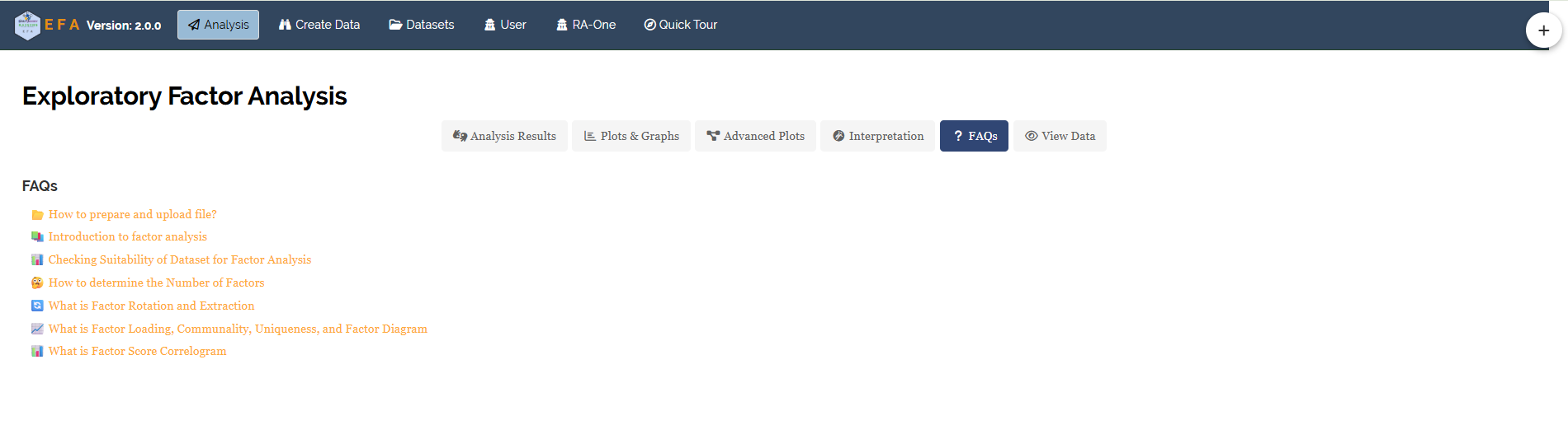
Frequently asked questions
How many factors should I retain? Read the four criteria together, as described in Section 9. When they agree, the decision is straightforward. When they disagree, fit the competing solutions and retain the most interpretable one.
A variable does not load on any factor. What should I do? A variable with no loading above 0.4 is not participating in the structure. Check its individual MSA in the KMO table and its communality. If both are low, it is measuring something of its own and is usually removed, after which the analysis is repeated.
What is a Heywood case? A communality of 1 or above, which is impossible for a proper solution because a variable cannot have more than all of its variance explained. RAISINS issues a warning when this occurs. It usually indicates that too many factors have been extracted, or that two variables are almost perfectly collinear. Reduce the number of factors and run the analysis again.
Why did the factor numbers change when I repeated the analysis? If an oblique rotation was used, the ordering of the factors is not guaranteed to be stable between runs. See the note in Section 2.
Should I use EFA or PCA? See Section 1.1 for a fuller comparison. In short, Principal Component Analysis reduces variables into components that capture as much total variance as possible and is a data-reduction technique, while Exploratory Factor Analysis models the shared variance in order to infer the latent causes of the correlations. Use EFA to explain why variables correlate, and PCA when the objective is simply fewer variables. RAISINS provides a separate module for PCA.
17 View Data
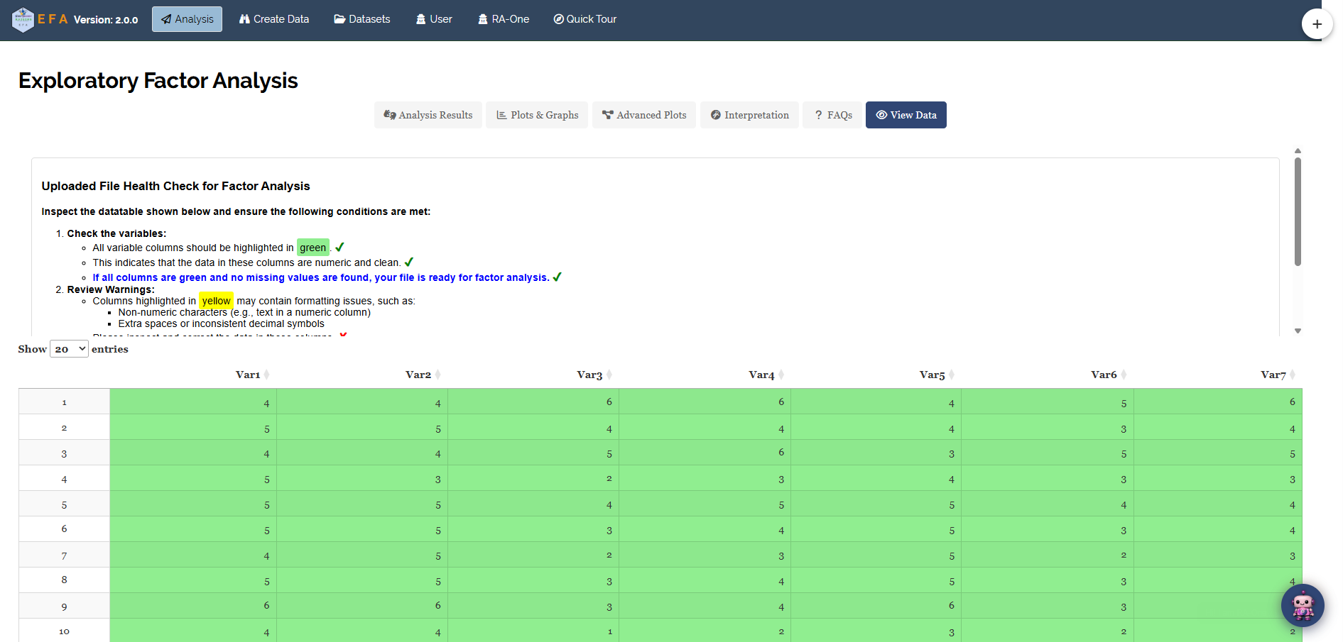
The View Data sub-tab displays the file exactly as RAISINS has read it. It is the first place to check when a result is unexpected, because most surprising output can be traced to a column that was not imported as intended.
18 Summary
The analysis of Dataset 1 established that the data were suitable for factor analysis, with a KMO of 0.814 and a significant Bartlett’s test. Four independent criteria agreed on retaining 2 factors, which together explained 79.8% of the total variance.
The solution showed textbook simple structure. Var3, Var4, Var6 and Var7 defined the first factor and Var1, Var2 and Var5 the second, with no cross-loadings, communalities between 0.723 and 0.877, reliabilities of 0.942 and 0.917, and essentially perfect model fit. A supplementary oblique run confirmed that the two dimensions are effectively independent (factor correlation = −0.034).
What remains is the part the software cannot supply: deciding what the two dimensions represent in the context of your research, and whether that interpretation is defensible. Exploratory Factor Analysis establishes that the structure exists. Naming it, and reporting it correctly, is the researcher’s responsibility.
19 Appendix: A Short History of Factor Analysis
Factor analysis originated in the study of human intelligence in the early twentieth century. In 1904 Charles Spearman, a British psychologist and statistician, observed that different measures of cognitive ability tended to correlate with one another. He proposed that a single general intelligence factor, which he called g, could account for these shared correlations, and he developed the foundations of factor analysis in order to test the idea formally.
The method was substantially extended over the following decades. Thurstone introduced multiple-factor solutions and the concept of simple structure, arguing that a good solution should have each variable loading strongly on as few factors as possible. These developments allowed factor analysis to spread beyond psychology into sociology, marketing, ecology and agricultural research, wherever a large set of measured variables needed to be reduced to a manageable number of underlying dimensions.
Exploratory Factor Analysis, as distinguished from its confirmatory counterpart, remains the most widely used variant when the researcher has no prior hypothesis about the factor structure and wishes to allow the data to reveal its own organisation.
If you have any doubt please feel free to contact us at [email protected]. Our statisticians are there to help you. HAPPY STATISTICS with STATOBERRY!