Kruskal-Wallis Test
The Kruskal-Wallis test compares three or more groups on a numeric response without assuming normality or equal variances, working on ranks instead of raw values. This tutorial explains the H-statistic, why a significant result only means “some group differs,” how Dunn’s test and LSD post-hoc comparisons and compact letter grouping pin down which groups differ, and how to run the whole analysis code-free… Read more …
The Kruskal-Wallis test is the nonparametric, rank-based alternative to a one-way ANOVA for comparing three or more independent groups on a numeric response, used when the data are ordinal, the sample is small, the distributions are skewed, or normality and equal variance simply cannot be assumed. Because it works directly on ranks rather than raw values, it needs no data transformation.
This tutorial introduces the basic concepts behind rank-based testing, including how the Kruskal-Wallis H-statistic is formed, what a significant omnibus test does and does not tell you, and how post-hoc pairwise comparisons and compact letter grouping identify which specific groups differ. It then provides a step-by-step guide to performing the analysis in the RAISINS platform: preparing your data, running the test, choosing between Dunn’s test and LSD as the post-hoc method, reading every part of the results table, reviewing the thirteen available plots, and using the built-in RA-One AI assistant to interpret the output. No programming knowledge is required.
1 What is the Kruskal-Wallis Test?
Suppose a panel of judges scored four rice varieties on overall appearance, on a 1-5 scale, with ten judges tasting each variety. You want to know whether the varieties differ in how they were scored. A one-way ANOVA would be the obvious first choice, but ANOVA assumes the scores within each variety are approximately normally distributed and that the four varieties have roughly equal variance. A 1-5 rating scale from ten judges is exactly the kind of data where that assumption is shaky: the scores are ordinal rather than truly continuous, ties are common (several judges giving the same score of “4”), and the distribution of a small sample is easy to get wrong by eye.
The Kruskal-Wallis test sidesteps the assumption entirely. Instead of analysing the raw scores, it first pools every observation from all four varieties together and converts every score to its rank, from lowest to highest, across the whole combined dataset, ties receiving the average of the ranks they span. It then asks a simple question: if the four varieties were really identical, would you expect their groups’ rank totals to be this different, or would you expect them to be roughly equal? The test statistic, usually called H, measures how far the observed group rank totals are from what equal groups would produce. Under the null hypothesis of no group difference, H follows an approximate chi-squared distribution with k − 1 degrees of freedom, where k is the number of groups, and RAISINS reports the corresponding p-value.
Because the test works on ranks rather than raw values, it does not need the response to be normally distributed, and it is far less sensitive to a handful of extreme scores than ANOVA is. The trade-off is that a rank-based test generally has slightly less statistical power than ANOVA when ANOVA’s assumptions genuinely hold; you gain robustness, not a free upgrade.
The Kruskal-Wallis test converts a numeric response, pooled across three or more groups, into ranks, and asks whether those ranks are distributed unevenly across the groups, without requiring the response itself to be normally distributed or the groups to have equal variance.
Reach for Kruskal-Wallis instead of a one-way ANOVA whenever one or more of the following apply: the response is ordinal rather than truly continuous (rating scales, scores out of ten, judge panels); the sample size is small, making it hard to check normality with any confidence; the distribution is visibly skewed, with a long tail in one direction; the groups show clearly unequal variances; or you simply cannot verify the normality assumption and would rather not gamble on it. None of this makes Kruskal-Wallis a universal replacement for ANOVA. When the assumptions genuinely hold, ANOVA extracts more information from the same data.
The Kruskal-Wallis test is not simply a test for “different medians,” despite frequently being described that way. It formally tests whether the rank distributions of the groups differ. This is equivalent to a difference in medians only when every group’s distribution has the same shape and spread, differing only in location. If the groups’ distributions differ in shape, skewness, or spread, a significant Kruskal-Wallis result can occur even when the medians are identical, and conversely two groups with different medians can, in unusual cases, fail to register as significant. Treat a significant result as evidence that the groups’ distributions differ somewhere, and inspect the plots (Section 9) before writing “the medians differed” in a manuscript.
2 Which Groups Differ?
A significant Kruskal-Wallis result answers only one question: at least one of the groups differs from at least one other. It is an omnibus test, exactly like the F-test in a one-way ANOVA, and it does not say which pair, or how many pairs, are responsible for the significant result. With four rice varieties, a significant H could mean V1 alone stands apart from the other three, or that all four differ from each other, or anything in between. Answering “which groups differ” requires a second step: a post-hoc pairwise comparison, run only after the omnibus test itself is significant at the chosen significance level.
RAISINS offers two post-hoc methods, selectable from a dropdown:
- Dunn’s test (the default), computed via
FSA::dunnTest(). It compares every pair of groups using the pooled rank variance from the overall test, and is the standard, widely cited post-hoc procedure to pair with Kruskal-Wallis. Its p-value adjustment method is itself selectable: none (the default), bonferroni, sidak, holm, hs, hochberg, bh, or by. - LSD (least significant rank difference), computed via
agricolae::kruskal(group = TRUE). It compares mean ranks pairwise using a rank-scale analogue of Fisher’s LSD, familiar to anyone who has used the equivalent option in RAISINS’ ANOVA-based modules. Its own p-value adjustment method is selectable separately: none (the default), holm, hommel, hochberg, bonferroni, BH, BY, or fdr.
Whichever method you choose, the outcome is condensed into a compact letter grouping: each group is assigned one or more letters, and any two groups that share at least one letter are not significantly different from each other. For Dunn’s test, RAISINS assembles the full matrix of pairwise adjusted p-values, orders the groups by descending mean rank so that “a” marks the highest-ranked group, and passes the matrix to multcompView::multcompLetters(). For LSD, the letters come directly from agricolae::kruskal()’s own grouping output, which uses the same “highest rank gets a” convention. Either way, the letters give you, at a glance, exactly what the raw pairwise p-value table would otherwise require careful reading to establish.
Dunn’s test is the more conservative and more widely reported choice for Kruskal-Wallis post-hoc comparisons in the literature, and is a reasonable default for most agricultural and biological work, especially with an adjustment method such as bh (Benjamini-Hochberg) or bonferroni if you are running many comparisons and want to guard against false positives. LSD is more liberal (closer in spirit to an unadjusted pairwise comparison) and tends to detect more differences, at some cost in the false-positive rate; it will feel familiar if you already use LSD-based grouping in RAISINS’ ANOVA modules.
The Level of significance (α) dropdown, 0.05 (default) or 0.01, applies to both the omnibus Kruskal-Wallis test and, when it runs, the chosen post-hoc method. A stricter α = 0.01 requires stronger evidence before the omnibus test is judged significant, which also means the post-hoc comparison and its letter grouping will only be computed when that stricter bar is cleared.
3 Getting to the Module
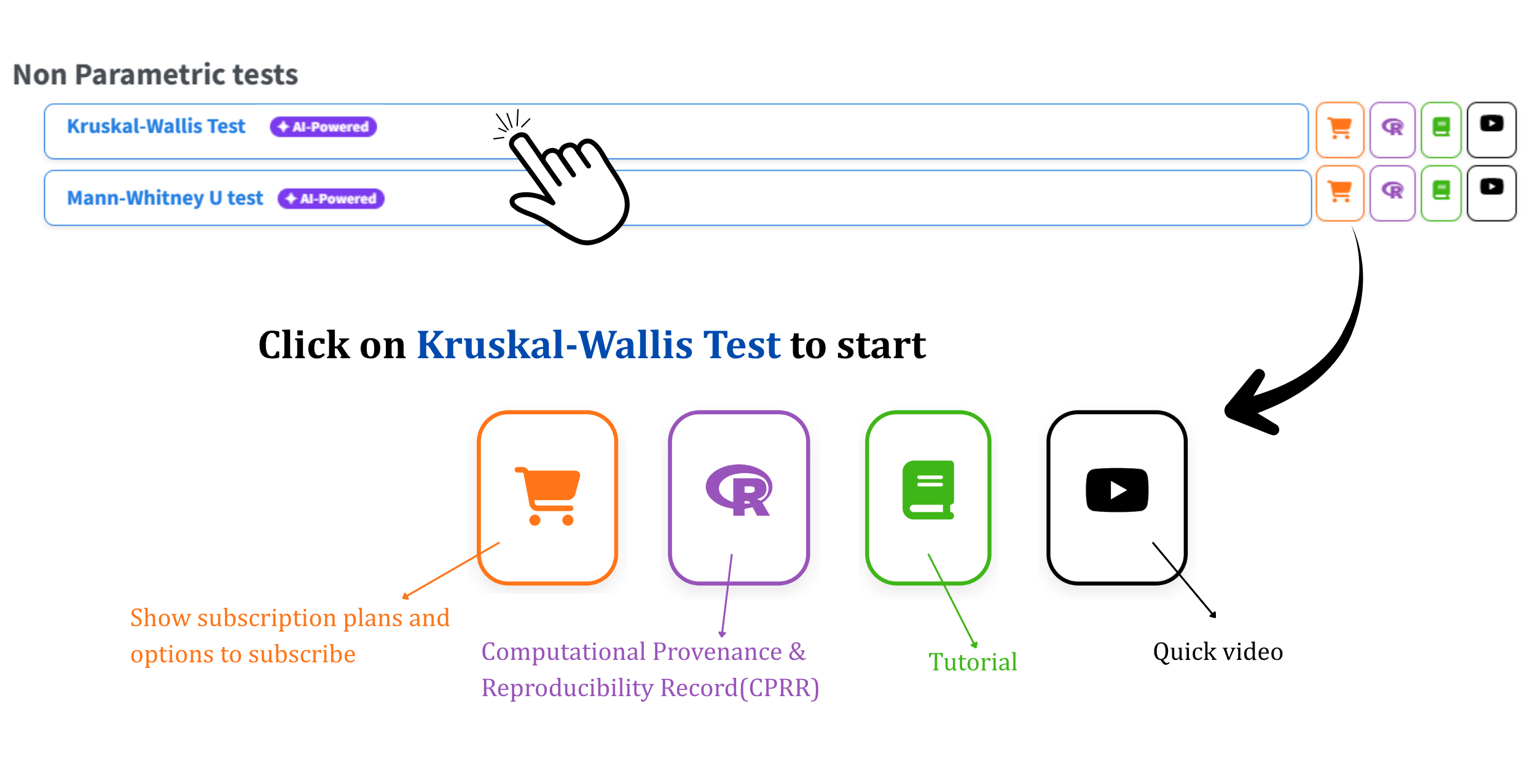
Open the RAISINS home page at www.raisins.live and go to the Non-Parametric test section. Select the Kruskal-Wallis Test module (Figure 1).
No programming knowledge is required. You upload your data, select the grouping column and one or more response variables, and RAISINS performs the complete analysis, from the omnibus test through the post-hoc comparison and compact letter grouping, and produces publication-ready output.
3.1 Computational Provenance & Reproducibility Record
CPRR (Computational Provenance & Reproducibility Record) provides a transparent and comprehensive record. Click on the icon shown in Figure 1 to access CPRR and know about the computational workflow performed during the analysis. The record for this module states the R version and the exact version of every package used, names the specific function behind each reported result. CPRR lists every default parameter and decision rule applied by the module and provides fully runnable R code that reproduces each analytical step. Users can execute the code in R to independently reproduce and verify the results. It carries its own DOI.
To cite the platform itself in a paper, thesis, or report, use the RAISINS citation, available in APA, Harvard, and BibTeX formats at www.raisins.live/citation.html. That is the primary reference, and for most manuscripts it is all you need.
The CPRR for the Kruskal-Wallis Test module is at www.raisins.live/module_record/kwt.html.
Cite the RAISINS paper as your primary reference for the platform. Add the CPRR as supporting documentation when a journal asks for details of the computing environment, or when you want your methods section to be precise about versions and functions rather than saying “analysis was carried out using an online tool.” The CPRR supports the citation and ensures computational reproducibility.
4 Preview Mode and Quick Tour
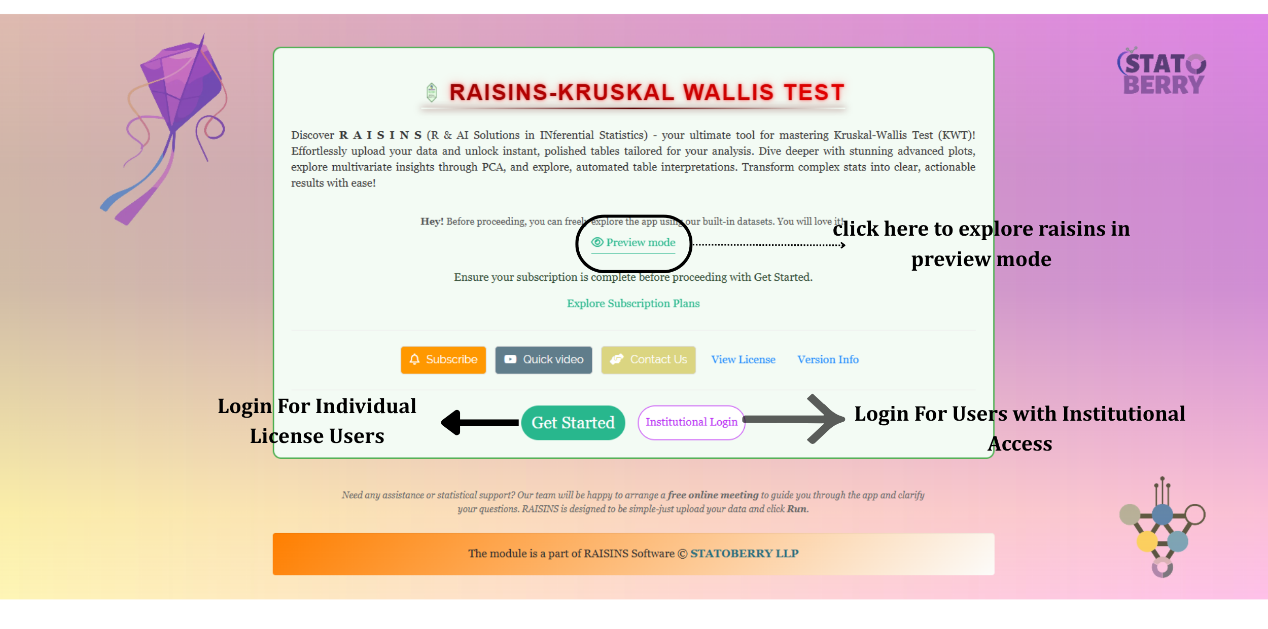
You can explore the entire module before subscribing by using Preview mode on the Welcome page. It loads the built-in demo datasets, so you can try every feature, including the analysis, the post-hoc comparisons, and all thirteen plots, without uploading your own data.
On first login, you are also offered a choice between Take the tour and Skip. Taking the tour launches an interactive, guided walkthrough that highlights each navbar tab and sidebar control in turn and explains what it does, from uploading a file all the way through to downloading a report. You can replay it at any time from the Quick Tour tab in the top navigation, whether or not you took it the first time.
5 The Example Dataset
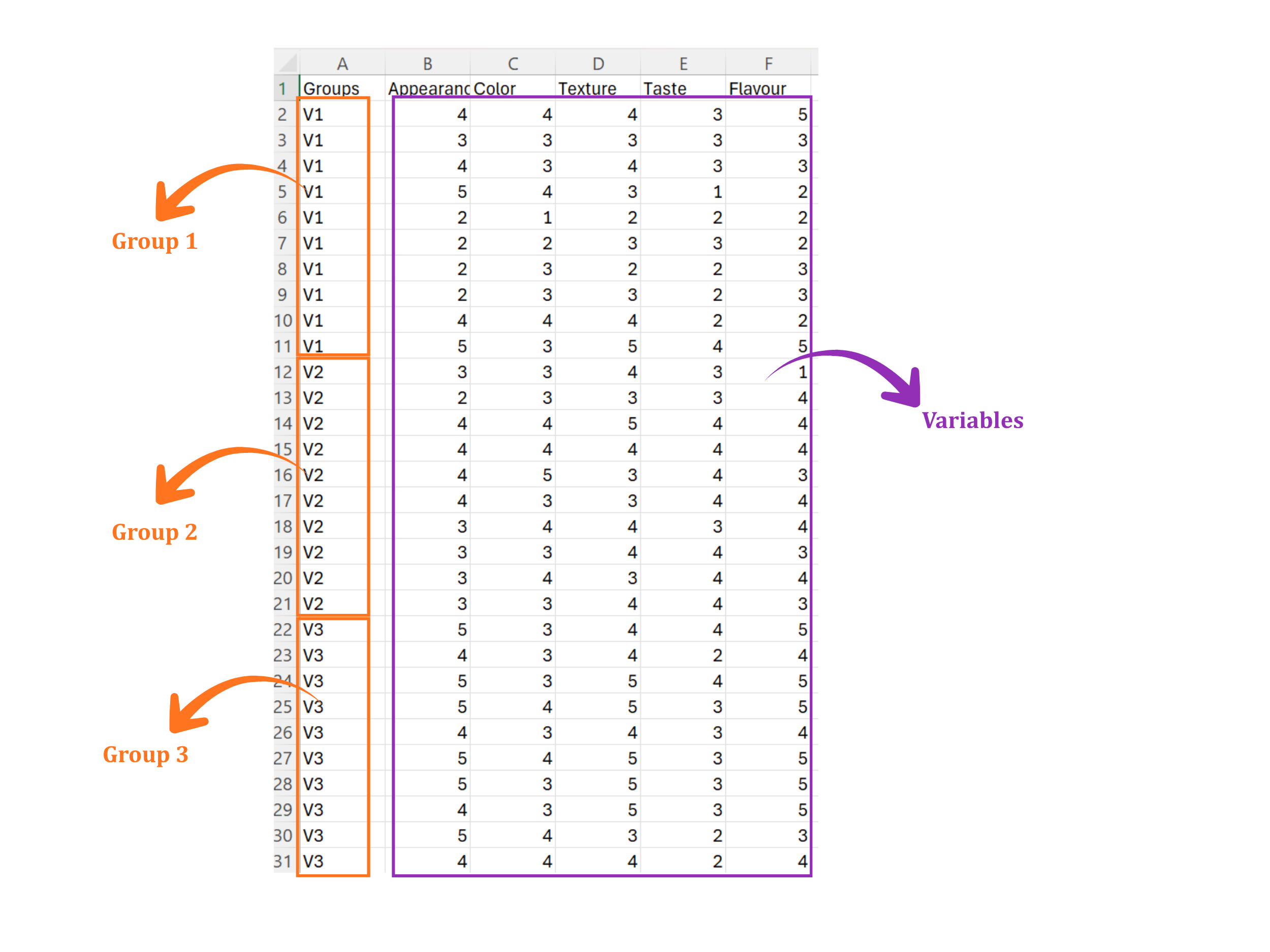
This tutorial uses the built-in dataset1.csv, a sensory evaluation of four rice varieties, labelled V1 through V4, available from the Datasets tab. Ten judges rated each variety, giving 40 rows in total (10 replications per variety), on five response variables, each scored on a 1-5 scale:
- Appearance
- Color
- Texture
- Taste
- Flavour
The data are laid out with a Groups column first, holding the variety label (V1-V4), followed by the five response columns, one per sensory attribute (Figure 3).
This kind of data is arguably a better fit for Kruskal-Wallis than for a one-way ANOVA. Judge ratings on a bounded 1-5 scale are ordinal, cluster into a handful of repeated integer values (producing many tied ranks), and rarely resemble a smooth normal curve, especially with only ten judges per variety. Rather than transforming the scores or hoping the ANOVA assumptions hold well enough, the rank-based approach works with the data exactly as collected.
- Prepare your dataset.
- Upload the data.
- Select the Treatment (grouping) column and one or more Response Variables.
- Choose the post-hoc method, p-adjustment, significance level, and digits.
- Run the analysis.
- Examine the Kruskal-Wallis H-statistic, p-value, and compact letter grouping.
- Review the plots.
- Read the automatic interpretation, or ask RA-One.
- Export the downloadable report.
The sections below walk through each of these steps in detail.
6 Preparing Your Data
The quality of your analysis depends on the quality of your data. RAISINS provides four ways to prepare a correctly formatted dataset:
- Create it in MS Excel.
- Build it inside the app using Create Data.
- Download a built-in Model dataset and use it as a reference.
- Generate it through the RA-One chat assistant.
6.1 Preparing Data in MS Excel
Open a new Excel workbook containing a single sheet. Arrange the data in columns: one column for the Treatment (grouping) variable, listing which group each observation belongs to, followed by one column for each numeric response variable. Each row represents one observation. Every response column must contain only numeric values; the Treatment column holds the group labels.
Save the file in CSV, XLS or XLSX format. CSV is recommended because it is smaller and loads faster. Avoid blank rows above the data and extra spaces in column names. Refer to Figure 3 for the required layout.
Dataset creation rules
- Column naming - do not use spaces. Use underscores (
_) or dots (.), and avoid symbols such as % and #. Always begin a column name with a letter. - Data arrangement - start at the upper-left corner of the sheet. The row above the data must not be blank.
- Cell management - do not type or delete in empty cells. If needed, select them, right-click, and choose Clear Contents.
- Column relevance - give every column a meaningful name, and remove columns you will not analyse.
- Numeric response columns only - every response variable column must contain only numbers. Entries such as “NA” or ” - ” will cause errors. The Treatment column is the only column allowed to hold text/categorical labels.
How to save as CSV in MS Excel
- Open your workbook, with the data on a single sheet and correctly arranged.
- File → Save As / Save a Copy, then choose a location.
- Save as type → CSV (Comma delimited) (*.csv).
- Name the file without spaces. Use underscores instead.
- Save.
💡 Tip: before saving, confirm that the data is on the first and only sheet, that the Treatment column comes first, and that every response column is numeric.
6.2 Creating Data Inside RAISINS
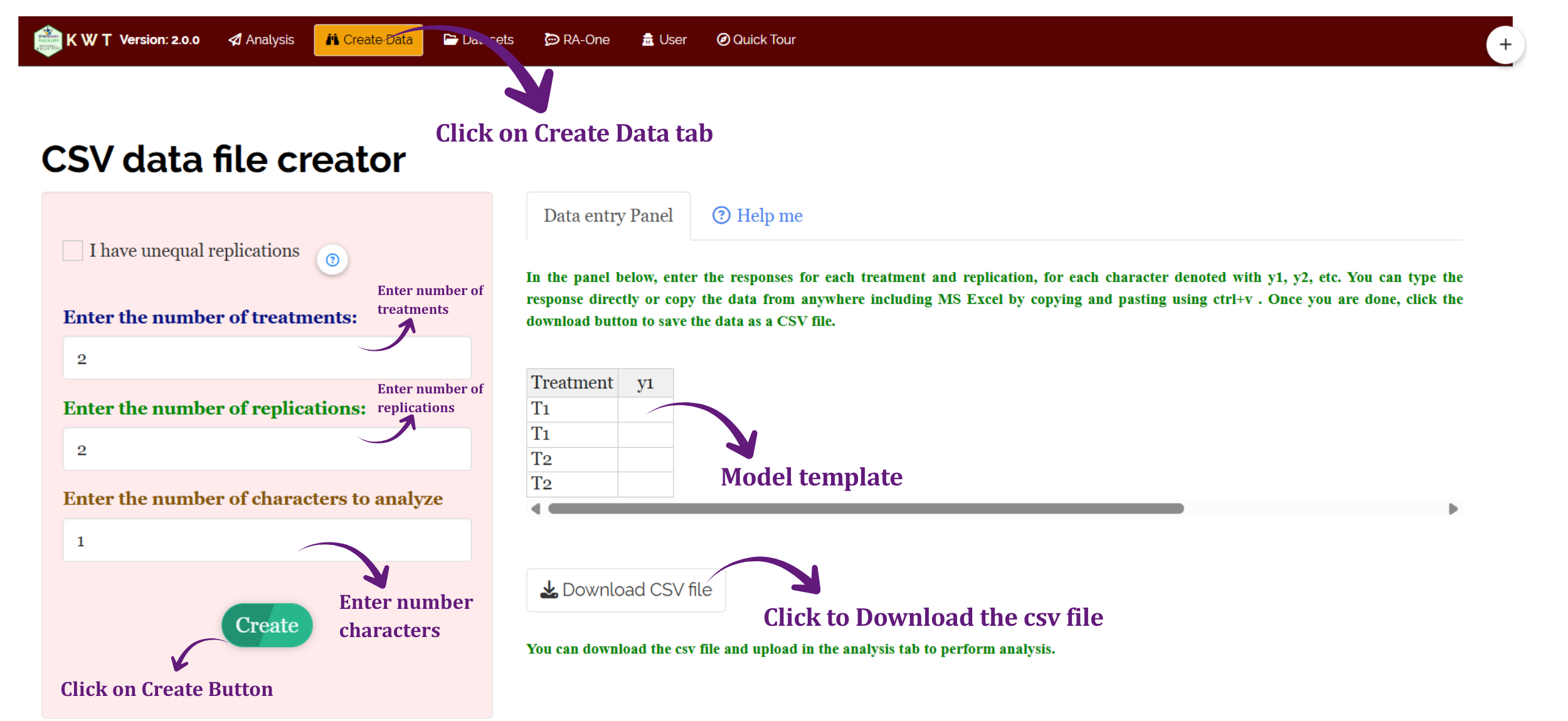
If you are unsure about the required format, RAISINS can generate a template for you without writing a single line of code:
- Go to the Create Data tab.
- Select the number of Variables.
- Select the number of Observations, which is the number of rows.
- Click Create.
The generated layout is shown in Figure 4. Enter your values in the template directly or download the template as a CSV file and enter the values in the downloaded CSV file, then upload it in the Analysis tab.
6.3 Downloading Model Datasets
To explore the module before using your own data, download a ready-made example:
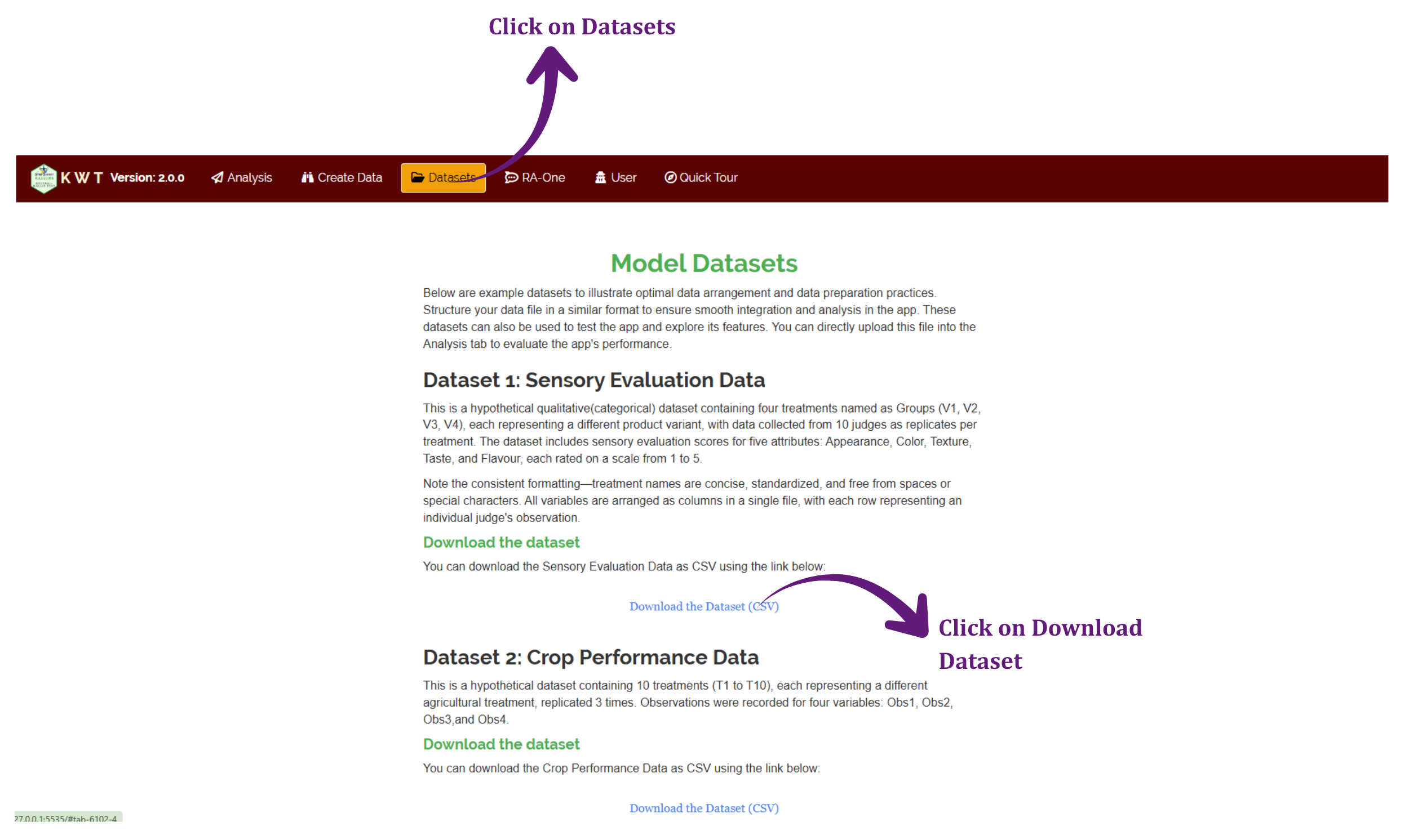
- Go to the Datasets tab.
- Click the Download CSV link for the dataset you want. Two model datasets are bundled: dataset1.csv (4 rice varieties, 5 sensory response variables, used throughout this tutorial) and dataset2.csv (10 treatments, 4 numeric response variables).
- Use it as a formatting reference, or upload it directly to run the analysis.
6.4 Creating a Dataset Using RA-One
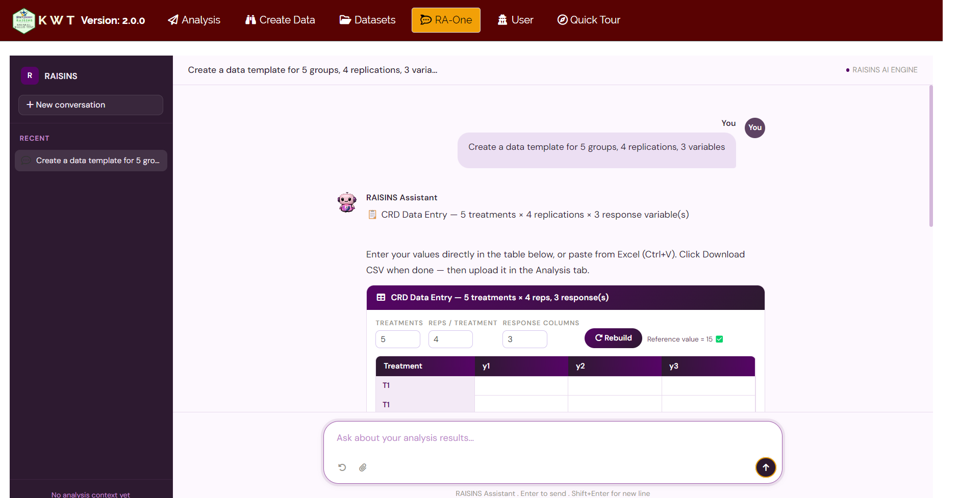
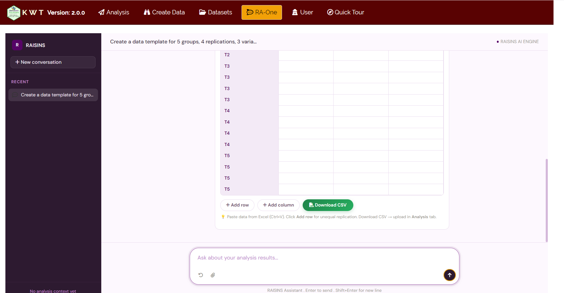
RA-One, the built-in chat assistant, can create a correctly formatted dataset through a simple conversation.
Open RA-One from its navigation tab or from the floating chat bubble. Tell it how many groups, how many response variables, and how many observations you need, and it generates a template in the required format, Treatment column first, response columns after. Review the template in the chat, download the CSV file, and upload it in the Analysis tab (Figure 6).
7 The Analysis Tab
The top-level navigation of the module runs Welcome, Analysis, Create Data, Datasets, RA-One, User, Quick Tour, in that order. Everything from here through Section 16 happens inside Analysis, which is itself organised into eight subtabs, shown as pills across the top of the page: Analysis.Results, Basic Plots, Advanced Plots, Summary stats, AI interpretation, Multivariate, FAQs, View Data. This tutorial covers each of these in turn, in a slightly more logical reading order than their left-to-right position on screen.
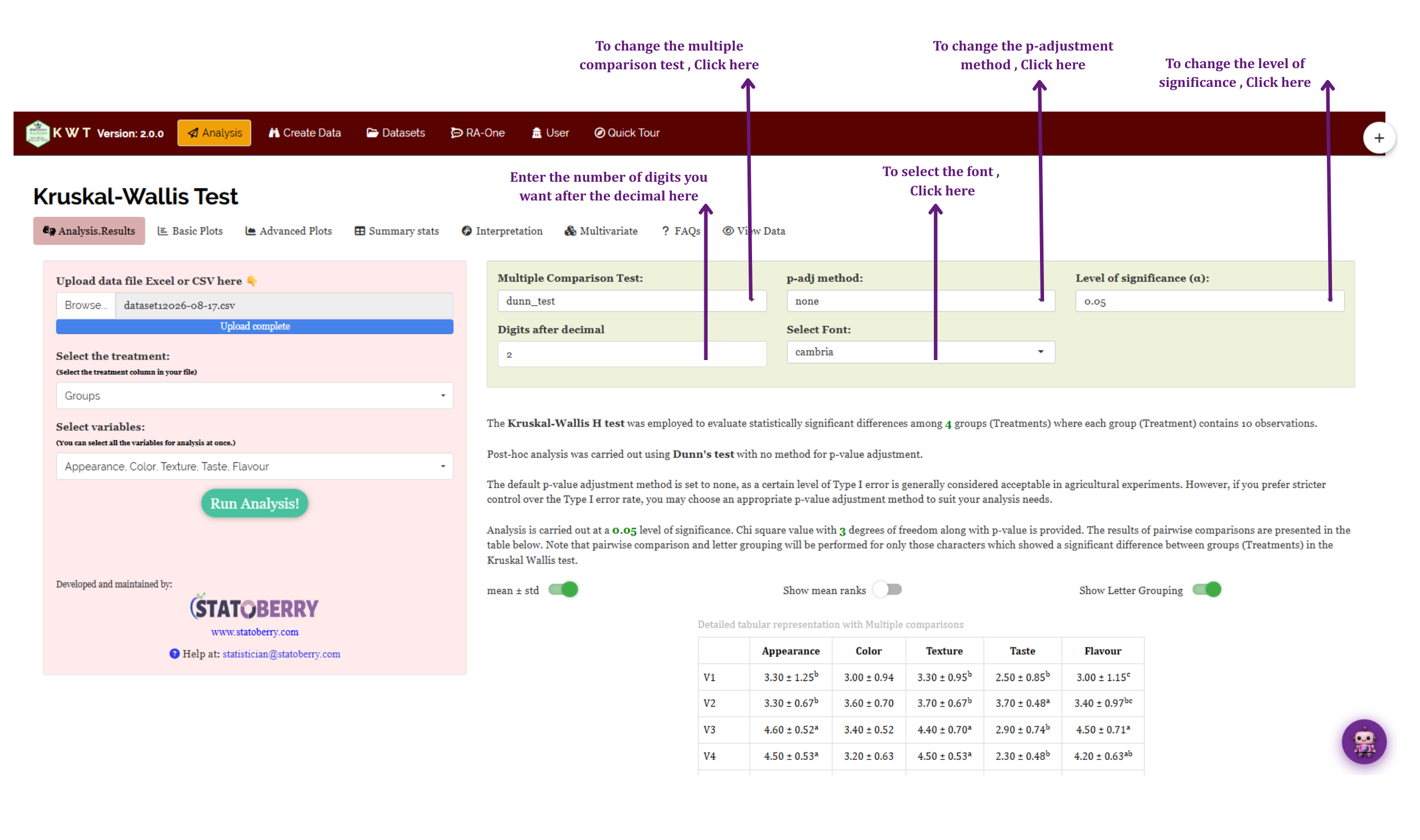
The Analysis.Results subtab, is where the Kruskal-Wallis test is fitted (Figure 7).
Click Browse in the sidebar to upload your CSV or Excel file. Two selectors then appear:
- Treatment - a single-select picker for the grouping column (for the worked example, Groups).
- Response Variable(s) - a multi-select picker for one or more numeric columns to test. Whichever column is chosen as Treatment is automatically removed from the choices offered here.
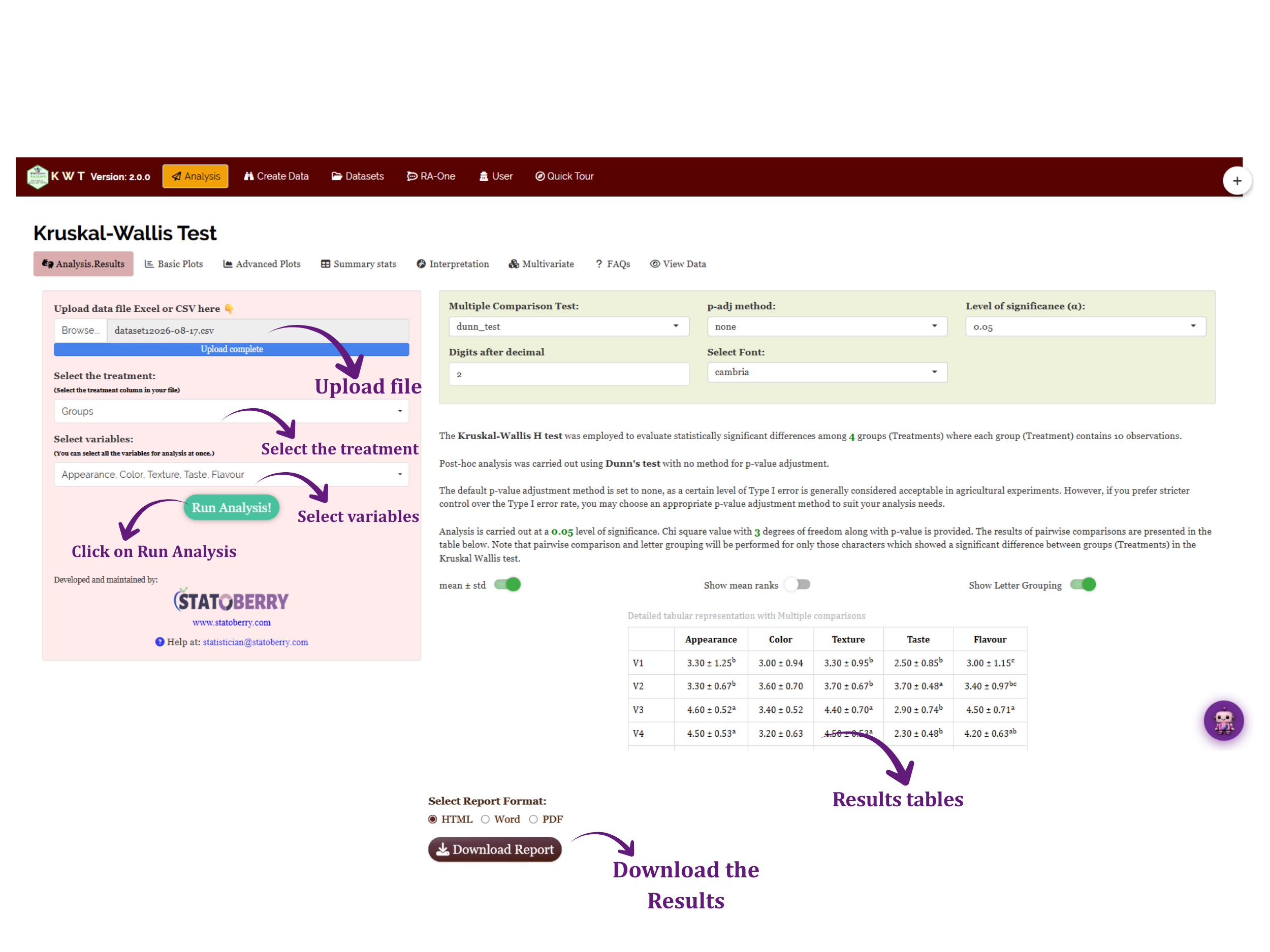
A settings row above the results table lets you control how the test is run and how the table is displayed:
- Multiple Comparison Test - Dunn’s test (default) or LSD, as explained in Section 2.
- P-adjustment method - the list offered depends on which post-hoc test is selected: none/bonferroni/sidak/holm/hs/hochberg/bh/by for Dunn’s test, or none/holm/hommel/hochberg/bonferroni/BH/BY/fdr for LSD. none is the default for both.
- Level of significance (α) - 0.05 (default) or 0.01, used for the omnibus test and to gate whether the post-hoc comparison runs at all.
- Digits - the number of decimal places shown in the output tables, default 2.
- Font - the font used to render the results table.
- Three display toggles, described in full in Section 8: mean ± std, Show mean ranks, and Show Letter Grouping.
Every one of these updates the displayed results immediately; there is no separate “Run Analysis” step to repeat after changing a setting once the test has been run the first time.
If the Kruskal-Wallis H-test for a response variable is not significant at the chosen α, RAISINS does not compute a post-hoc comparison or a letter grouping for that variable; every group is, statistically, indistinguishable from every other, so there is nothing for a pairwise test to resolve. Switching the significance level from 0.01 to 0.05 (or back) can change which response variables receive a post-hoc comparison, without needing to re-upload or re-select anything.
Two of the eight subtabs extend beyond the results table itself, but use the same uploaded file: Summary stats (Section 10), the per-group distribution tables, and Multivariate (Section 11), a PCA-based index-scoring tool. Both are covered in their own sections below.
8 Analysis Results
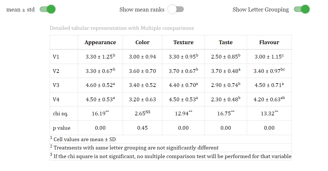
The Analysis.Results subtab presents a single results table covering every selected response variable at once: one column per response variable and one row per group (a level of the Treatment column), with two further rows, chi sq. and p value, appended at the bottom carrying the omnibus test result for each column. Above the table, a short written summary states how many groups were compared, whether replication was equal, which post-hoc test and p-adjustment were used, the significance level, and the degrees of freedom.
8.1 Reading the omnibus statistics
For each response variable, RAISINS reports the H-statistic (the chi-squared approximation from kruskal.test()) and the p-value in the last two rows of the table, with a significance star on the chi-square figure: ** when p ≤ 0.01, * when p ≤ 0.05, and NS (not significant) otherwise. The degrees of freedom (number of groups minus one) is the same for every column and is stated once, in the written summary above the table, rather than repeated in each column.
One point to keep in mind: the stars use the conventional fixed thresholds of 0.01 and 0.05, whereas the letter grouping is gated on the significance level you selected. If you set α to 0.01 and a variable returns p = 0.03, its chi-square will still be starred * while no letters are produced for that column, because at your chosen α the omnibus test did not reach significance.
8.2 The three display toggles
A row of three toggles sits directly above the results table and controls how each group’s row is displayed, independently of the underlying computation:
- mean ± std - switches each group’s cell between showing the mean alone and showing mean ± standard deviation, both computed on the raw, unranked values within that group.
- Show mean ranks - appends each group’s mean rank (in parentheses) alongside the mean/mean ± SD figure. The mean rank is what the Kruskal-Wallis test itself operates on, so this is the most direct way to see, numerically, why the letters fell the way they did.
- Show Letter Grouping - shows or hides the compact letter grouping superscripts described in Section 2, together with their explanatory footnote, in both the on-screen table and, as covered in Section 14, the downloadable report.
Reading a finished row: a group displayed as, for example, “3.85 ± 0.49a” with the mean rank “(28.4)” on the line beneath it - all three toggles on - means a mean Appearance score of 3.85, a standard deviation of 0.49, a mean rank of 28.4 among all 40 judges’ ratings, and a letter grouping of “a”, meaning this variety sits in the top rank-tier and is not statistically distinguishable, at the chosen α, from any other variety also carrying an “a”. A variety carrying only “b” would be significantly lower-ranked than every “a”-only variety; a variety carrying “ab” overlaps with both tiers and is not significantly different from either.
The significance stars answer “does this response variable differ across groups at all.” The compact letter grouping answers “which specific groups differ from which.” A response variable can be highly significant overall (H-test, **) while still having every group letter-linked to at least one neighbour, meaning no single pairwise comparison alone reaches significance once you split the overall effect across all of the pairs. Report both figures, not just the star.
9 Plots and Graphs
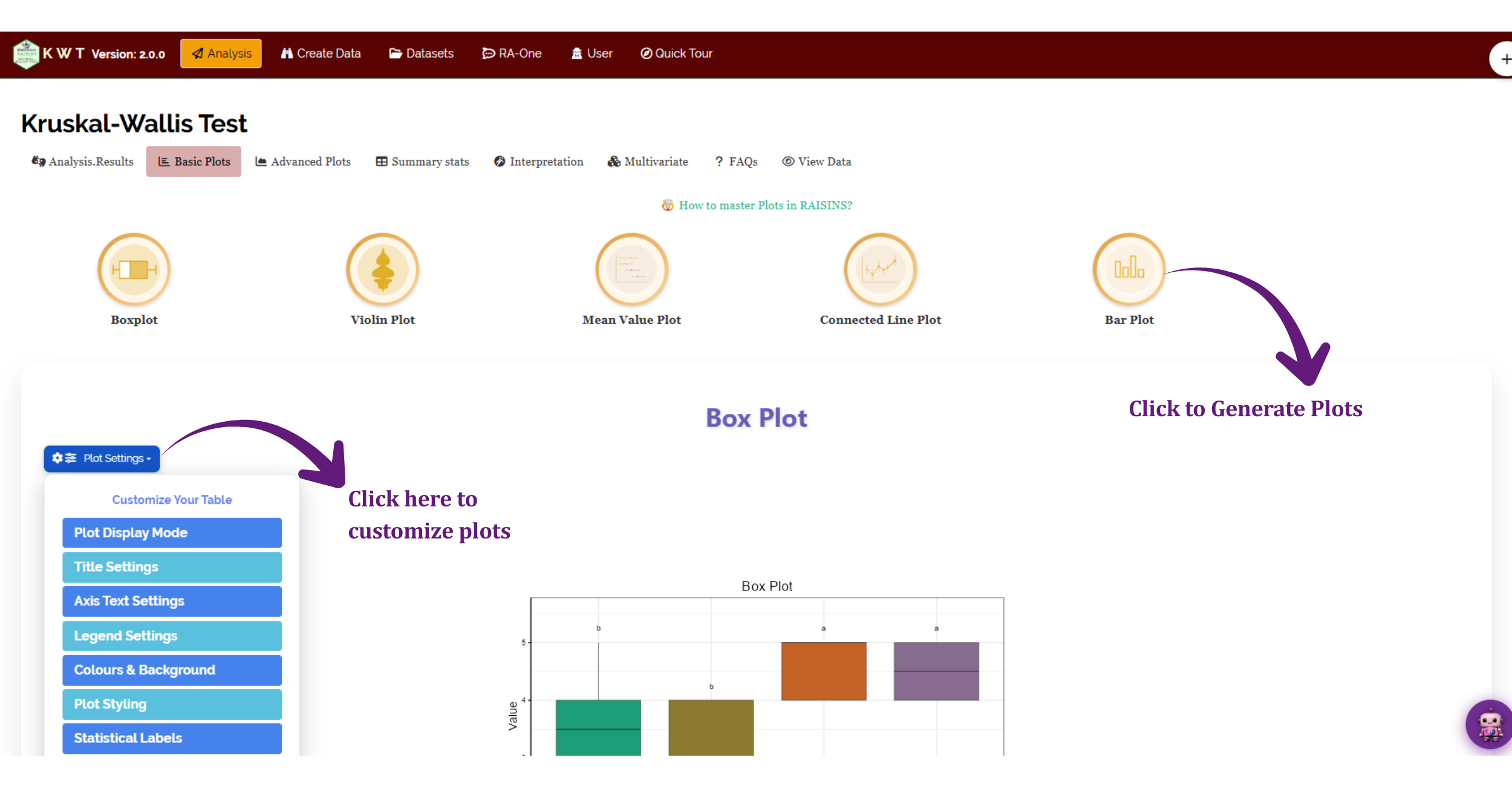
The Basic Plots and Advanced Plots subtabs together offer thirteen visualizations, selected using a row of icon buttons, split across the two subtabs by complexity. The five comparison plots that can display compact letters (Boxplot, Violin, Mean Value, Connected Line, Bar) are built from the same per-group summary statistics and the same letter grouping used in the results table, so a letter or a value shown in a plot always traces back to the identical underlying computation; the remaining panels are diagnostic or exploratory views of the same uploaded data. Every plot can be customized (title, axis labels, colours, theme) through a gear-icon Plot Settings panel, and downloaded at a resolution you choose.
9.1 Basic Plots
- Boxplot (Figure 11) - the standard summary of each group’s distribution: median, interquartile range, and outliers. The natural starting point for any group comparison, and a useful visual check on the “same shape” assumption behind reading a significant result as a median difference (Section 1).
- Violin Plot - a boxplot with the full estimated density drawn around it, showing whether a group’s ratings are unimodal, bimodal, or piled up at one end of the scale, detail a boxplot alone cannot show.
- Mean Value Plot - each group’s mean plotted as a point with a horizontal ± 1 SD error bar, the most compact view for a quick group-to-group comparison. Note that the error bars are always the standard deviation of the raw values, while the compact letters above them come from the rank-based post-hoc test (Section 2); the two answer different questions, so a group can carry the higher letter without having the longer bar.
- Connected Line Plot - group means connected by a line in Treatment order, useful when the groups have a natural sequence, such as increasing levels of a factor, even though Kruskal-Wallis itself treats the groups as unordered categories.
- Bar Plot (Figure 12) - group means as bars, the most familiar chart type for a non-technical audience, such as a thesis committee or a field-day poster.


9.2 Advanced Plots
- Summary - not a chart but a summary table, one row per column of the data you selected, with an inline mini-histogram alongside that column’s missing count, mean, median, and standard deviation. A single-glance data-quality overview before drilling into any one plot.
- Raincloud - a “cloud” (density), “rain” (individual points), and boxplot layered together, one panel per response variable. Note that this panel pools all treatments together: it shows the overall distribution of each variable, not a group comparison. Use the Advanced Raincloud below for that.
- Advanced Raincloud (Figure 13) - the same cloud/rain/box layering, but drawn per treatment for one selected response variable, with optional median labels. This is the most informative single view of a Kruskal-Wallis result, because it shows the medians the test is comparing along with every raw observation behind them.
- Circular (Figure 14) - treatment means arranged around a circular axis, one segment per response variable. By default each variable is min-max normalized so variables measured on different scales can share the same rings; that means the lowest treatment of each variable is drawn at zero height rather than at a zero value, and the subtitle on the figure says so. Unticking Scale data plots the raw means on their own scale instead.
- QQ (Figure 15) - a quantile-quantile plot of the response, checking visually how far each distribution departs from a normal curve, a useful diagnostic for confirming that reaching for Kruskal-Wallis instead of ANOVA was the right call. Panels can be drawn per treatment, as a treatment × variable grid, or with the treatments combined; optional confidence bands and normality-test p-values (Shapiro-Wilk, Anderson-Darling, and the Lilliefors-corrected Kolmogorov-Smirnov) can be annotated on each panel. When the treatments are combined into a single panel, the values plotted are centred on their own treatment median, so what you are judging is the within-treatment residuals rather than the group differences.
- Distribution (Figure 16) - like Summary, a table rather than a chart: one row per treatment, with an inline distribution sparkline (density, histogram, or boxplot, your choice) for every response variable, so the shapes can be compared treatment by treatment at a glance.
- Pair - pairwise scatter plots across every selected response variable, coloured by group, with the correlation coefficient shown in the upper panels, useful when more than one response variable was selected.
- Correlation (Figure 17) - a correlation matrix across the selected response variables, showing which sensory attributes tend to move together (in the worked example, whether Taste and Flavour track each other, for instance). Because this module exists precisely for data that are not assumed normal, both this panel and the Pair panel default to Spearman’s rho, the rank-based coefficient; Kendall’s tau and Pearson’s r are also selectable.


If you only look at one plot, make it the Boxplot or the Raincloud. Both show the median, the spread, and (for the raincloud) every individual observation, which is exactly the information needed to sanity-check whether a significant Kruskal-Wallis result reflects a straightforward difference in location or a more complicated difference in shape (Section 1).
10 Summary Statistics
The Summary stats subtab gives the numbers behind the plots. It produces one table per response variable, headed by the variable’s name, with one row per treatment (Figure 18). For the worked example that means five tables, Appearance through Flavour, each with four rows for V1 to V4.
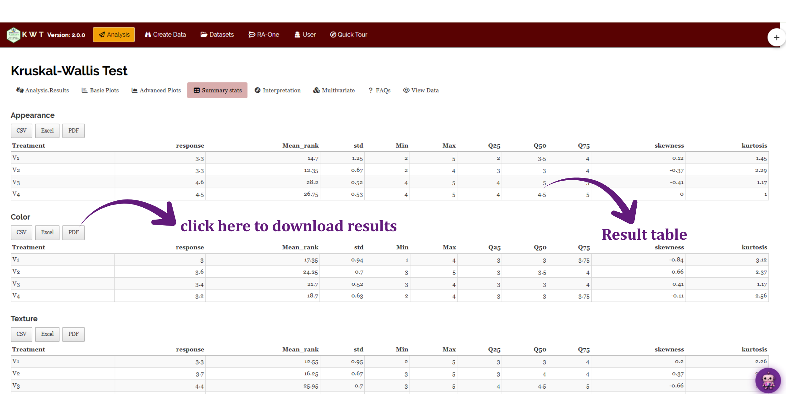
Each row carries eleven figures for that treatment:
- response - the group’s mean on that variable. The column keeps this generic name because the table is generated for whichever variable is being summarised.
- Mean_rank - the group’s mean rank. This is the quantity the Kruskal-Wallis test actually compares, so this column is the most direct numerical explanation of why the letters in Section 8 fell the way they did. A group with the highest mean rank is the one carrying “a”.
- std - the standard deviation of the raw values within that group.
- Min, Max - the smallest and largest observation in the group.
- Q25, Q50, Q75 - the first quartile, the median, and the third quartile. Q50 is the group median, which is what most write-ups quote alongside a Kruskal-Wallis result.
- skewness, kurtosis - the shape of the group’s distribution. Skewness near zero means roughly symmetric; a large positive value means a long right tail.
Above every table sit CSV, Excel and PDF buttons, so any single variable’s summary can be exported on its own without downloading the whole report.
Section 1 explains that a significant Kruskal-Wallis result only translates into “the medians differ” when the groups have a similar distribution shape. The skewness column is the quickest way to check that: if one group is strongly skewed while the others are symmetric, or the skewness values swing from clearly negative to clearly positive across groups, report your result as a difference in distributions rather than a clean difference in medians. Reading Q50 next to Mean_rank is also a useful sanity check, since the two orderings should broadly agree.
11 Multivariate: PCA-based Index Scores
The Multivariate subtab answers a different question from the rest of the module. Kruskal-Wallis compares your treatments one response variable at a time; if a variety wins on Taste but loses on Texture, the results table cannot tell you which variety is best overall. The Multivariate tab addresses that by collapsing all of your response variables into a single index score per treatment, using Principal Component Analysis.
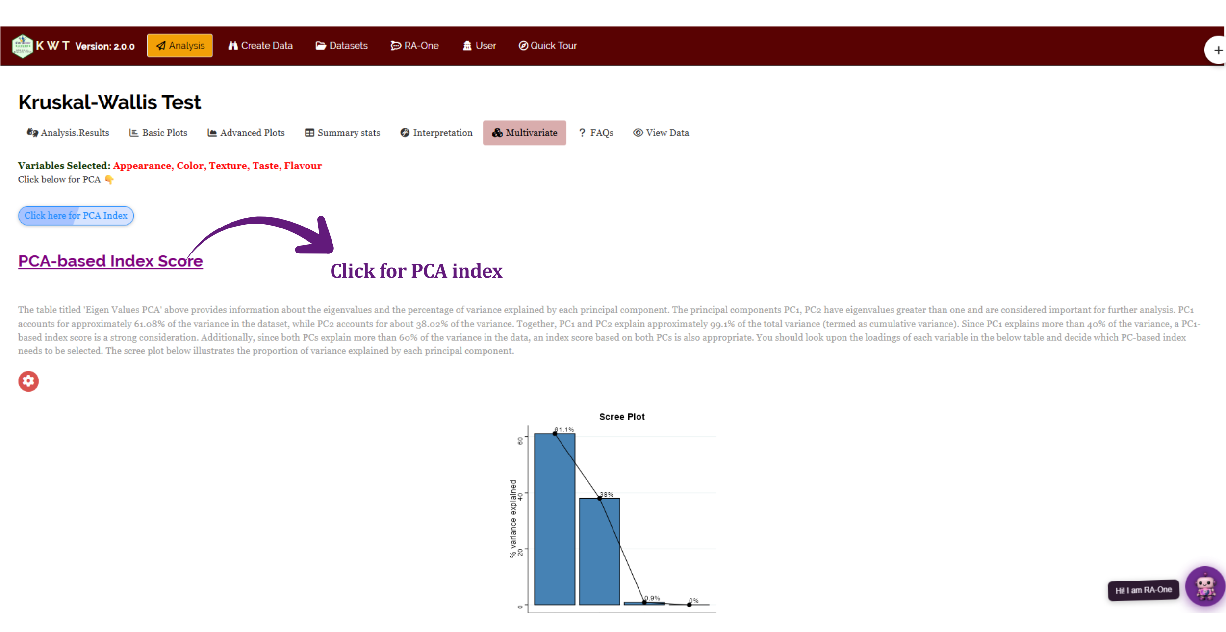
The tab needs at least three response variables — with fewer, it shows a message saying so instead. Click Click here for PCA Index to run it (Figure 19).
11.1 How the index is built
RAISINS first reduces your data to a matrix of treatment means, one row per treatment and one column per response variable, then runs PCA on that matrix with the variables centred and scaled to unit variance, so that a variable measured on a large scale cannot dominate one measured on a small scale. The tab then presents, in order:
- Eigen Values PCA - a table of eigenvalues with the percentage and cumulative percentage of variance explained by each component, followed by a short written commentary. In the worked example PC1 explains 61.1% and PC2 a further 38.0%, so the two together account for 99.1% of the variation among the varieties.
- Scree plot - the same information as a chart, for judging how many components are worth keeping.
- Loadings - how strongly each response variable contributes to each component. This is what tells you what the index means: if Taste and Flavour load heavily on PC1, then a PC1-based index is essentially a “flavour quality” score.
- Biplot - treatments and variable arrows on the PC1-PC2 plane, showing which treatments sit near which variables.
- Index score tables and plots - one set for PC1, one for PC2.
The commentary under the eigenvalue table makes this recommendation for you, using two thresholds: if PC1 explains more than 40% of the variance, a PC1-based index is a strong choice; if PC1 and PC2 together explain more than 60%, an index using both is also defensible. If the two components together explain less than 60%, the app says explicitly that a PC-based index should be used with caution — your variables are not reducible to one or two dimensions, and an index would hide more than it summarises. Read the loadings before accepting any of it, since an index is only meaningful if you can say what it represents.
11.2 Reading the index tables and plots
Each index table has two columns per treatment:
- Index Score - the treatment’s raw score on that principal component. It is centred on zero, so it can be negative, and its units are arbitrary.
- Scaled Index - the same score rescaled to a 0 to 1 range across the treatments, where 0 is the lowest-scoring treatment and 1 the highest. This is the column used for selection and for the plot.
Below the table, a Select cutoff for Scaled Indexscore dropdown (0.50, 0.75, 0.80, 0.90, 0.95; default 0.75) and a toggle control which treatments are flagged. With the toggle in its “top” position, treatments whose scaled index is above the cutoff are marked Selected; flipping it to “bottom” instead selects those falling below the mirrored cutoff, for when a low score is the desirable outcome. The circular index plot then draws every treatment around a polar axis, coloured by Selected or Nonselected, with a reference line at the cutoff. The same pair of controls, table and plot is repeated for the second component further down the tab.
Three things to keep in mind before putting an index score in a manuscript. First, it is computed from treatment means, not ranks, so it does not inherit the distribution-free protection that the Kruskal-Wallis test gives you. Second, no significance test is attached to it: a treatment ranked first on the index has not been shown to differ significantly from the second, and only the results table (Section 8) can support that claim. Third, PCA on a small number of treatments is unstable — with only four or five treatments the components are fitted to four or five points, and small changes in the data can reorder the index. Treat it as a screening and ranking aid that complements the group comparison, not as a replacement for it.
12 Interpretation
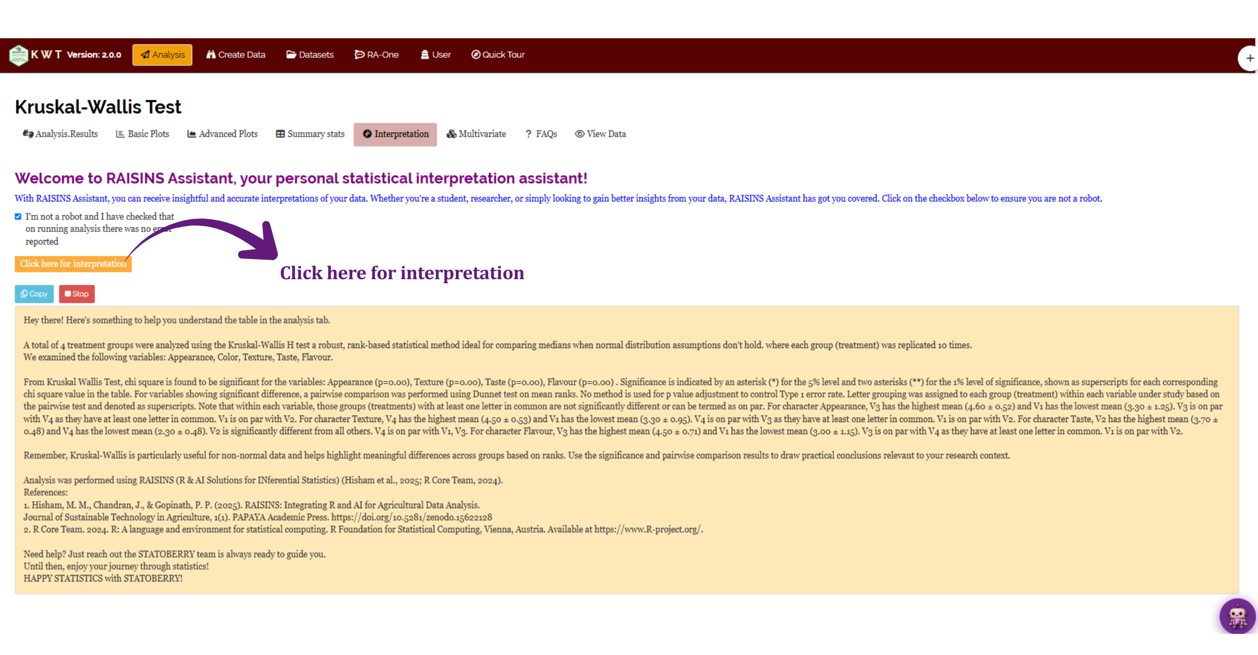
The AI interpretation subtab is an older, non-AI feature, kept alongside the newer RA-One assistant rather than replaced by it. It generates a canned, template-based written summary of the results in plain language (Figure 20): the H-statistic, the p-value, whether the test was significant, and which groups’ letters separate them from the rest.
The text appears with a short typewriter animation. A Stop button displays the full summary immediately, and a Copy button copies the plain-text version to your clipboard. Unlike RA-One (Section 13), this tab does not answer follow-up questions; it produces one fixed block of text per run.
13 RA-One Chat Assistant
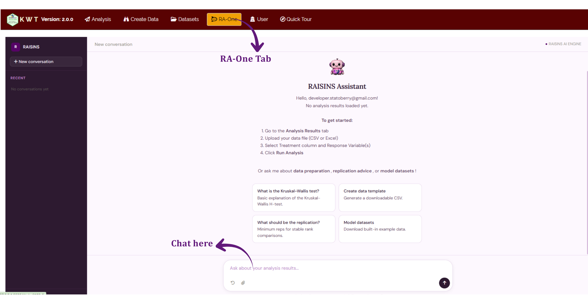
RA-One is the built-in chat assistant. You can open it from its navigation tab or from the floating chat bubble, visible once you are logged in.
Ask questions in plain language, and RA-One answers using your own analysis results. It does not give generic advice, and it does not invent values. If a value is not available, it says so. All replies are in plain English, with no code.
Before you have run an analysis, RA-One’s welcome screen offers four suggestion chips:
- What is the Kruskal-Wallis test? - a basic explanation of the Kruskal-Wallis H-test.
- Create data template - generates a downloadable CSV template in the required format.
- What should be the replication? - discusses the minimum number of replications needed for stable rank comparisons.
- Model datasets - offers dataset1.csv and dataset2.csv for download.
Once results exist, the chips change to match what you can now ask about:
- Interpret results
- Create data template
- Model datasets
- Report results - help writing up the results section of a manuscript or thesis.
RA-One has access to the complete set of results produced by the app: the H-statistic, degrees of freedom, and p-value for every selected response variable, the post-hoc comparison output and compact letter grouping (whichever method, Dunn’s or LSD, was selected), the per-group means, SDs, and mean ranks, and the dataset overview (sample size, groups, and response variables). You can ask it to explain what the H-statistic means for your specific results, why a particular pair of groups does or does not share a letter, or the difference between Dunn’s test and LSD.
RA-One can also prepare data and generate plots. It can build a correctly formatted data template (Section 6.4) or provide a model dataset (Section 6.3), and it can create any of the thirteen plot types described in Section 9 on request, for example “show me the raincloud plot for Taste” or “give me a boxplot”, with the figure displayed directly in the chat and a plot-type toolbar for switching between graph types without retyping the request.
When generating a data-entry template, RA-One applies a stability reference rather than the formal error-degrees-of-freedom rule used in RAISINS’ ANOVA-based modules. Kruskal-Wallis, being nonparametric, has no equivalent formal requirement on error degrees of freedom, so RA-One instead frames the familiar t(r-1) ≥ 12 rule of thumb (treatments × (replications-1)) as a practical guideline for how many replications tend to give stable, reproducible rank comparisons, not as a strict statistical requirement the test itself enforces.
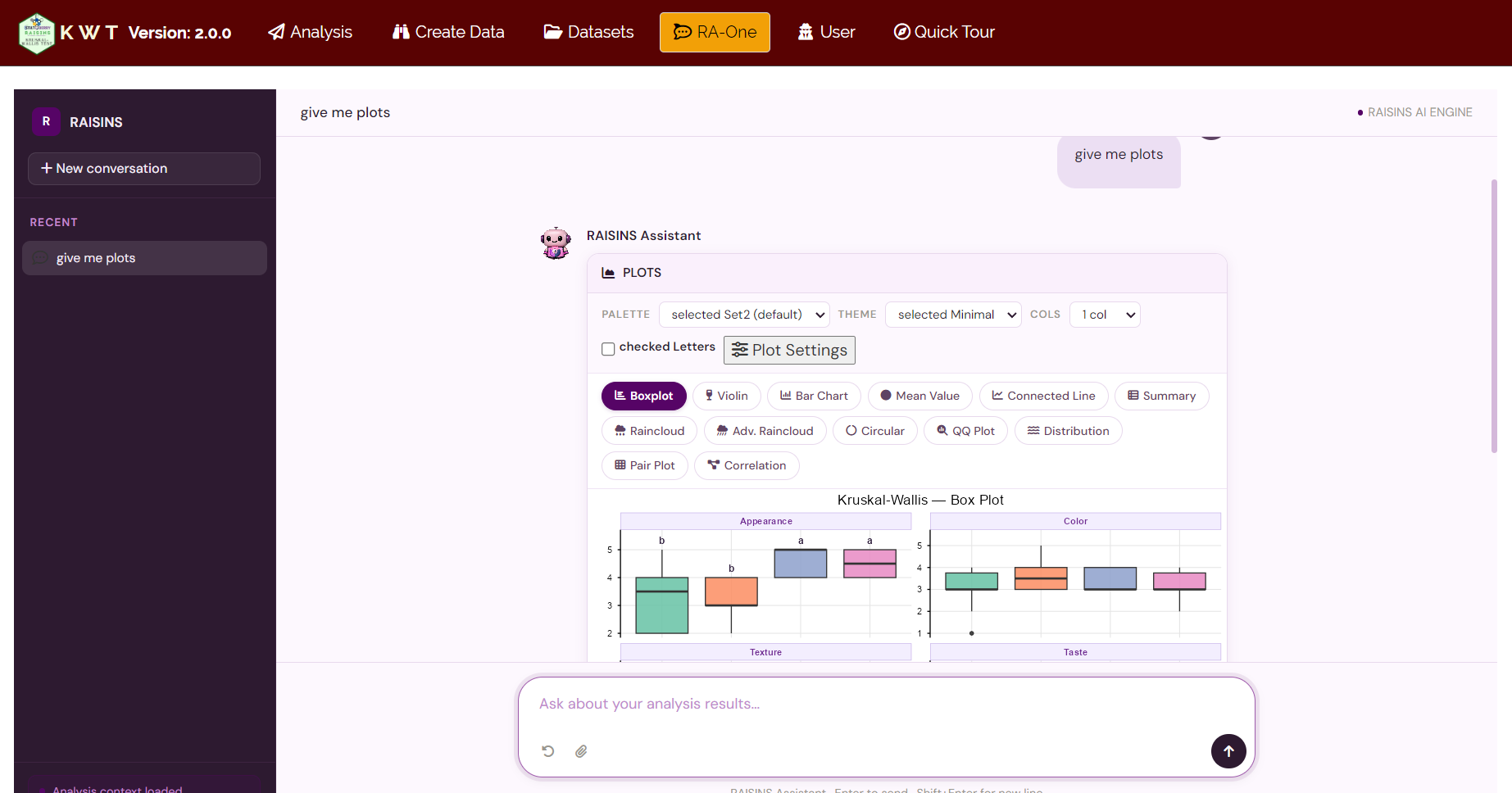
In a single conversation, RA-One can interpret your results, build a data template, provide a model dataset, and create any of the thirteen customizable plots. Much of a routine Kruskal-Wallis session can be completed without leaving the chat.
14 Downloadable Report
Below the results table in Analysis.Results, a Download Report control lets you export the complete set of results as a single document, in HTML, PDF, or Word format.
The report reproduces the same per-group table, omnibus statistics, and post-hoc grouping shown on screen for every selected response variable, so it can be attached directly to a manuscript or shared with a supervisor without copying each table by hand. Critically, the report respects whichever state the Show Letter Grouping toggle (Section 8) was in at export time: if the on-screen table is showing compact letters, the downloaded report shows them too, in the same format; if the toggle is off, the report omits them as well.
15 FAQs
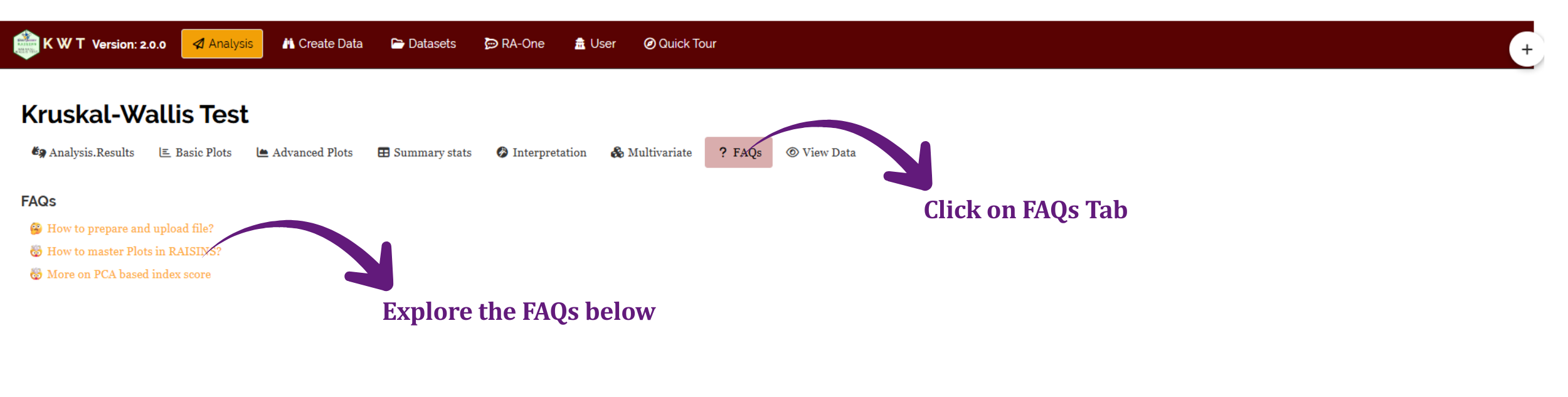
The FAQs tab answers common questions about the Kruskal-Wallis test and about the module itself. It covers topics such as when to prefer Kruskal-Wallis over a one-way ANOVA, how to choose between Dunn’s test and LSD, what it means when the omnibus test is significant but no pair of groups shows a letter difference, and how to interpret ties in the rankings.
If you are unsure how a feature works, start here.
16 View Data
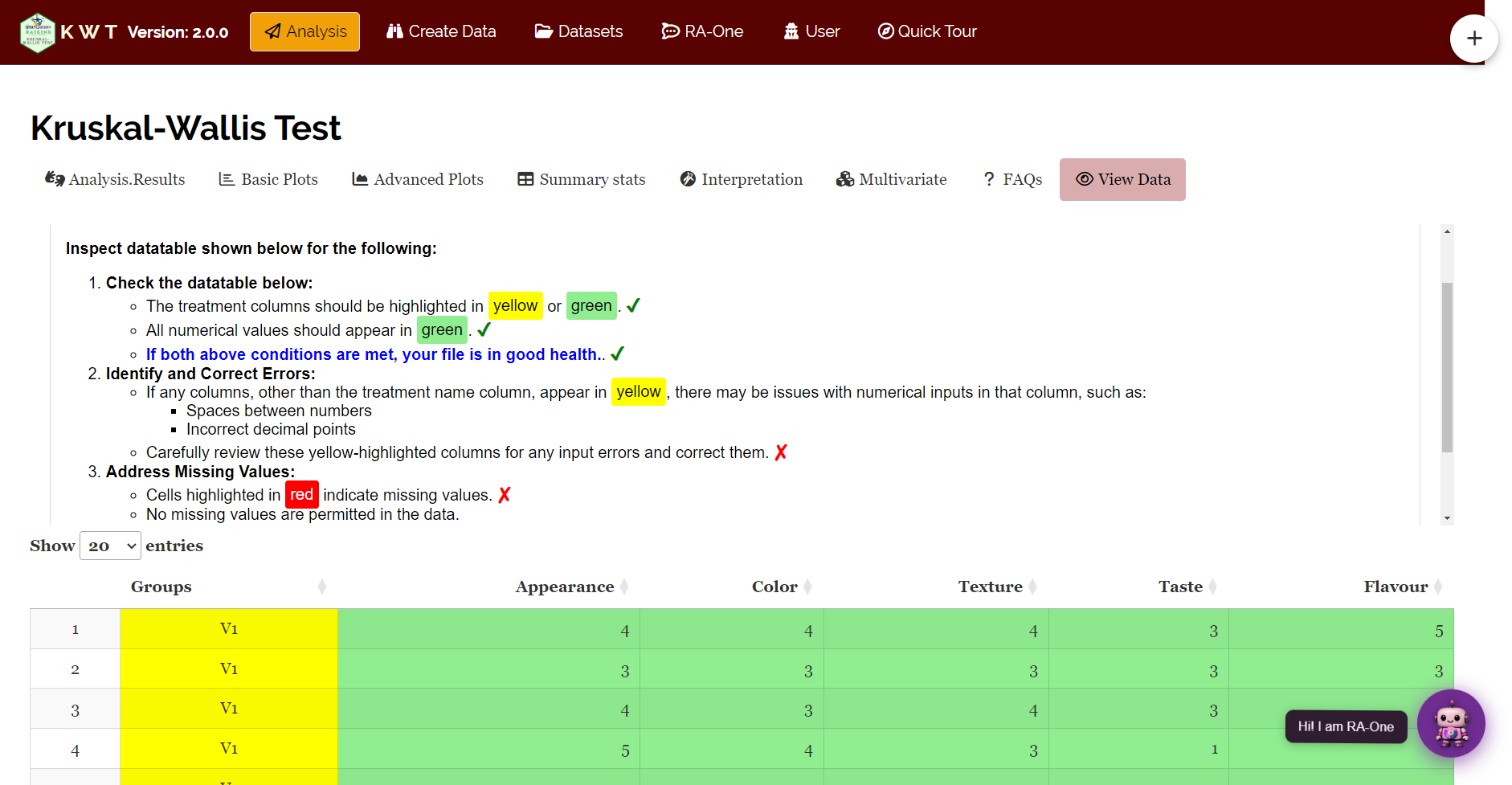
The View Data tab helps you confirm that your dataset is suitable for analysis.
When you upload a file, RAISINS runs an automated Health Check. It examines the column types and formatting, and flags any column that contains non-numeric values where a response variable is expected, missing entries, or inconsistent formatting.
Resolve any issues reported here before selecting your Treatment and Response Variable(s), so that your results are based on clean and correctly formatted data.
17 Summary
The Kruskal-Wallis test answers a single question: does the rank distribution of a numeric response differ across three or more independent groups, without requiring that response to be normally distributed or the groups to have equal variance?
Everything else in the output exists to make that answer complete and honest: the omnibus H-test to establish whether any difference exists at all, the post-hoc comparison (Dunn’s test or LSD) to identify which specific groups differ once it does, and the compact letter grouping that turns a matrix of pairwise p-values into a single glance-able label per group. RAISINS performs all of these calculations automatically, alongside thirteen plot types and a downloadable report, so you can concentrate on interpreting what the results mean for your research rather than on the mechanics of computing them.
If you need help at any stage, RA-One is available at all times. You can also write to us at [email protected].
18 Appendix: A Short History of the Kruskal-Wallis Test
The test was introduced by William Kruskal and W. Allen Wallis in their 1952 paper “Use of Ranks in One-Criterion Variance Analysis”, published in the Journal of the American Statistical Association. It generalised the two-sample Mann-Whitney U test (Mann & Whitney, 1947) to three or more groups, in much the same way that a one-way ANOVA generalises the two-sample t-test, but built entirely on ranks rather than on the raw measurements.
The test found rapid and lasting adoption in fields where distributional assumptions are routinely hard to defend, ordinal survey and rating data, small ecological and agricultural samples, and any dataset with visible skew or outliers, because it delivers a valid significance test without requiring the analyst to first verify normality. Olive Jean Dunn’s 1964 paper “Multiple Comparisons Using Rank Sums” supplied the pairwise post-hoc procedure now bearing her name, giving the omnibus test a standard way to localise a significant result to specific pairs of groups, the same procedure RAISINS offers as its default post-hoc method today.
Today, the Kruskal-Wallis test is a standard tool wherever a one-way comparison of three or more groups is needed but a one-way ANOVA’s assumptions cannot be relied upon, agricultural variety trials, sensory panels, and any small-sample or ordinal-response experiment among them.
