Line X Tester
Line × Tester Analysis (L×T) widely used for evaluating genetic potential in breeding populations… Read more …
Line × Tester analysis is a widely used mating design in plant breeding for evaluating the combining ability of parental lines and identifying superior hybrid combinations. It partitions genetic variation into General Combining Ability (GCA) and Specific Combining Ability (SCA), helping breeders understand additive and non-additive gene effects. In RAISINS, you can perform Line × Tester analysis effortlessly without writing a single line of code. This tutorial will guide you through the complete analysis workflow and help you interpret the results effectively. In addition, you will obtain ANOVA tables, GCA and SCA effects, variance components, genetic parameter estimates, publication-ready tables and plots, and AI-assisted interpretations for informed breeding decisions.
ABSTRACT
Line × Tester analysis is a mating design-based approach that crosses p lines with q testers to generate F₁ hybrids, enabling estimation of General Combining Ability (GCA) and Specific Combining Ability (SCA) through a structured ANOVA framework. GCA reflects additive gene action, while SCA captures non-additive effects including dominance and epistasis. The σ²GCA/σ²SCA ratio and Baker’s ratio determine the predominant gene action, guiding selection between population improvement and hybrid breeding strategies. In RAISINS, you can perform a complete Line × Tester analysis without writing a single line of code. This tutorial guides you through the analysis and interpretation of results. In addition, you will get publication-ready ANOVA tables, GCA and SCA effect estimates, heterosis statistics, rankings, and plots.
Hover or click each point to see more information.
Introduction to Line × Tester Analysis
-
The Line × Tester mating design was formalized by Kempthorne (1957)
 as a systematic method for evaluating combining ability in crop improvement programmes. The design involves crossing a set of female parents (lines) with a set of male parents (testers) to produce F₁ hybrids. The analytical procedure was further elaborated by Singh and Chaudhary (1979), whose computational method remains the standard reference in plant breeding. The design partitions genetic variance into General Combining Ability (GCA), attributed to additive gene action, and Specific Combining Ability (SCA), attributed to non-additive effects. This partitioning guides breeders in selecting parents for population improvement or hybrid variety development.
1 Statistical Genetics
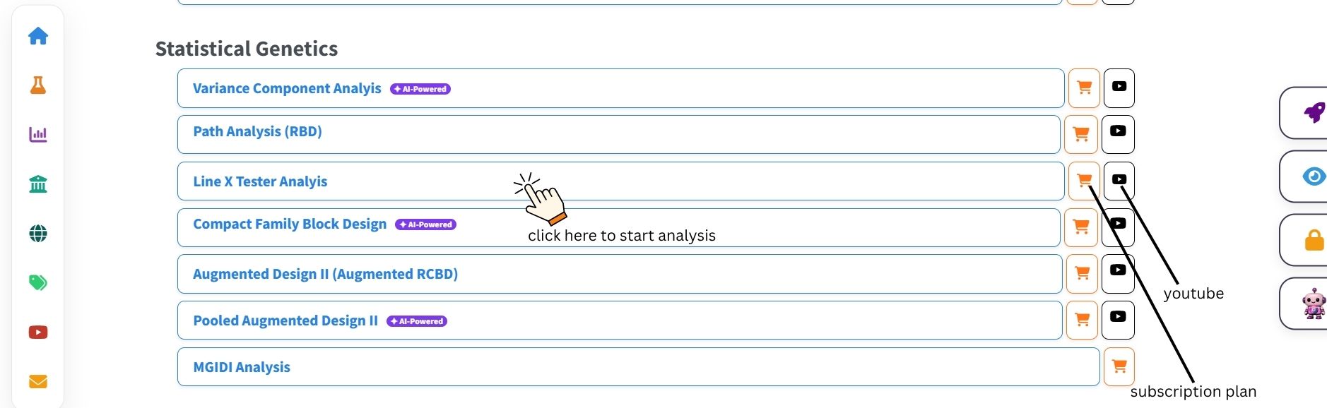
To get started, visit RAISINS www.raisins.live home page and go to Statistical Genetics. Here, you can see different mating design analyses available on the platform. In this tutorial, we focus on Line × Tester Analysis, as shown in Figure 1.
2 Line × Tester Analysis
Line × Tester analysis is a mating design in which p lines (female parents) are each crossed with q testers (male parents) to generate a set of p × q F₁ hybrid combinations. The hybrids, along with their parental lines and testers, are evaluated in a suitable experimental design - typically a Randomised Complete Block Design (RCBD). The statistical analysis partitions the total genetic variation into General Combining Ability (GCA) effects for lines and testers, and Specific Combining Ability (SCA) effects for individual cross combinations. This information is used to understand gene action, identify superior parents, and select promising hybrids for further evaluation or commercial release.
3 A Working Example
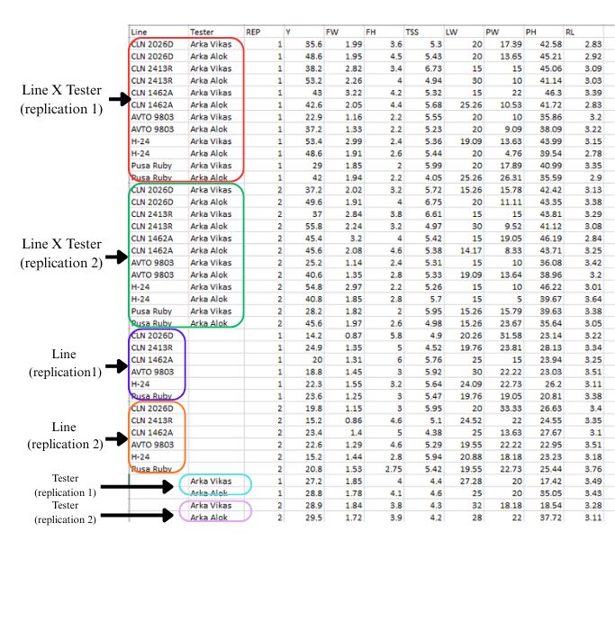
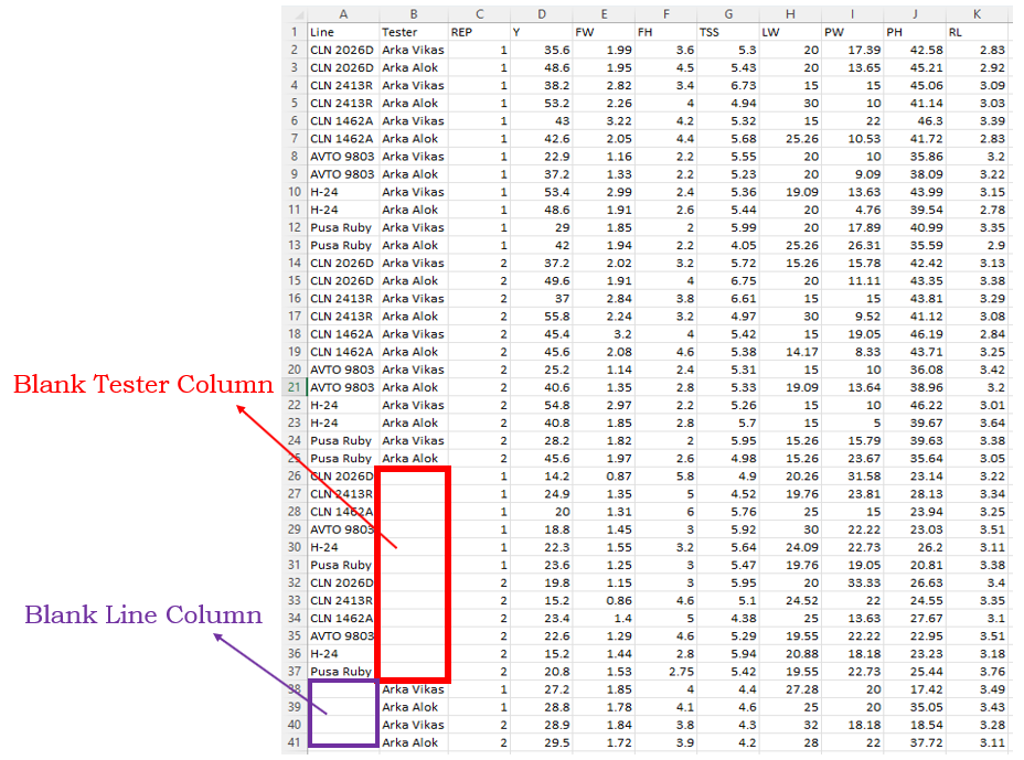
To make things simple and practical, we explain the Line × Tester analysis step by step using a real experimental example. Consider an experiment where 6 lines (CLN 2026D, CLN 2413R, CLN 1462A, AVTO 9803, H-24, and Pusa Ruby) are crossed with 2 testers (Arka Vikas and Arka Alok) to produce 12 F₁ hybrids. The hybrids along with their parents are evaluated in a Randomized Complete Block Design (RCBD) with two replications. Observations are recorded for several quantitative traits: Yield (Y), Fruit Weight (FW), Fruit Height (FH), Total Soluble Solids (TSS), Locule Width (LW), Pericarp Width (PW), Plant Height (PH), and Rind Length (RL). Our aim is to estimate combining ability parameters, identify good general and specific combiners, determine the nature of gene action, and compute heterosis statistics for each cross. The structure of the dataset is shown in Figure 2. Do not enter NA, dots (.), hyphens (-), numbers, spaces, or any symbols in the blank parent column - it must remain completely empty (Figure 3).
Data organized in MS Excel can be directly uploaded to RAISINS for analysis. For more details on data preparation, see Section 4 .Two terms used frequently are Lines, Testers, and Hybrids.
4 How to Prepare Your Data?
Arranging data for uploading in RAISINS is straightforward. Prepare your data exactly like Figure 3 using a single-sheet Excel file. Ensure no blank rows above the data and all columns have proper names. Your file is then ready to upload.
Still if you have doubt read below:-
To prepare your dataset for analysis in RAISINS, you have two options:
Creating dataset in MS Excel
Open a new Microsoft Excel file, use single sheet only.
Start with Cell A1: begin entering data from cell A1. Do not leave any blank rows above.
First Row - Column Names: The first row must contain the column names.
Column 1: Enter the Lines. Repeat the names according to the testers and replication.
Column 2: Enter the Testers. Repeat the names according to the lines and replication.
Column 3: Enter the replications.
From Column 4 Onwards: Enter the names of each variable under study as separate columns (e.g.Yield (Y), Fruit Weight (FW), Fruit Height (FH), Total Soluble Solids (TSS), Locule Width (LW), etc). You can give any names to the columns.
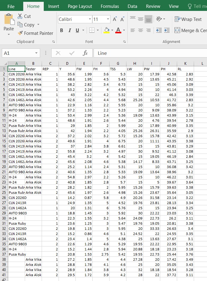
See Figure 2 showing how the prepared Excel file for upload should look like
If you have any doubt in saving a file as csv or some basics of data preperation read our tutorial on getting started here
Creating your dataset directly within the RAISINS app
Navigate to
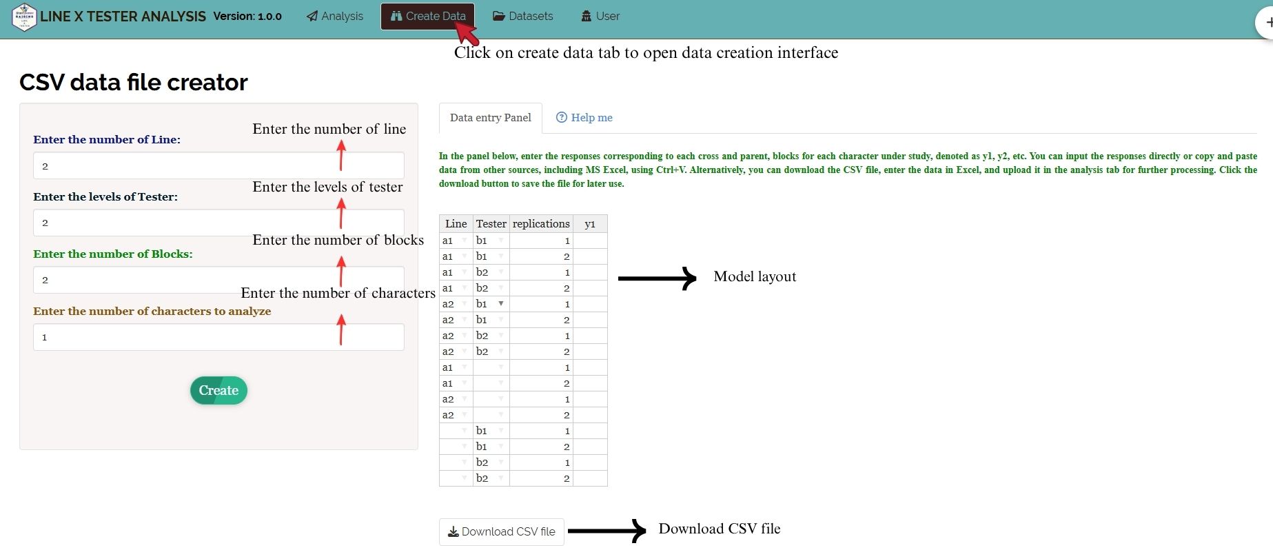
Create DataTab: Click on the Create Dataset tab in the main menu at the top of the app.Specify Details: Enter the number of Lines, Testers, Blocks and number of characters under study in the window that opens.
Then click
createModel Data Entry File: A template for data entry will be generated. You can:
Directly enter your data into this template.
Or, copy-paste data from an existing Excel file.
Download as CSV: Once the data is entered, click on the
Download CSVFile button. The downloaded CSV file can be uploaded for analysis inAnalysis tab.
5 Line × Tester Analysis Tab Explained
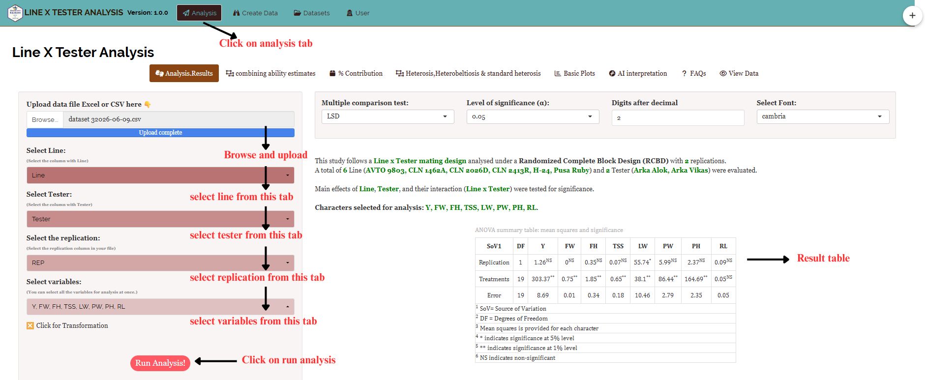
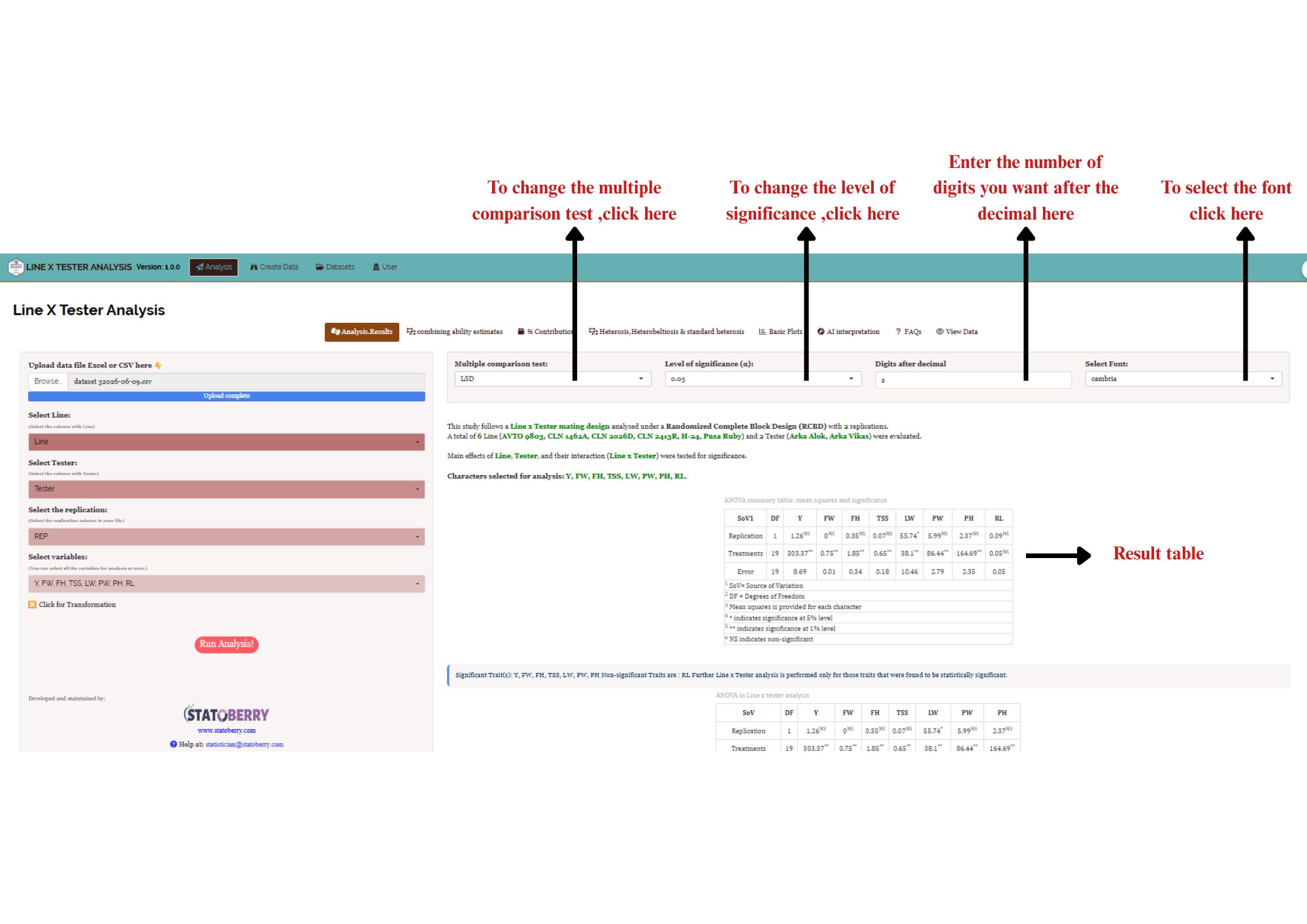
In Figure 4, you can see the detailed view of the Analysis tab along with explanations of what each option does. This section helps you understand the purpose of every setting, so you can select the most appropriate options for your data. Upload the prepared file by clicking Browse in the sidebar of the Analysis tab. When the file is uploaded, options to assign columns as Lines, Testers, Replication, and Variables will appear. Once you click the Run Analysis button, all relevant results and outputs appear instantly.
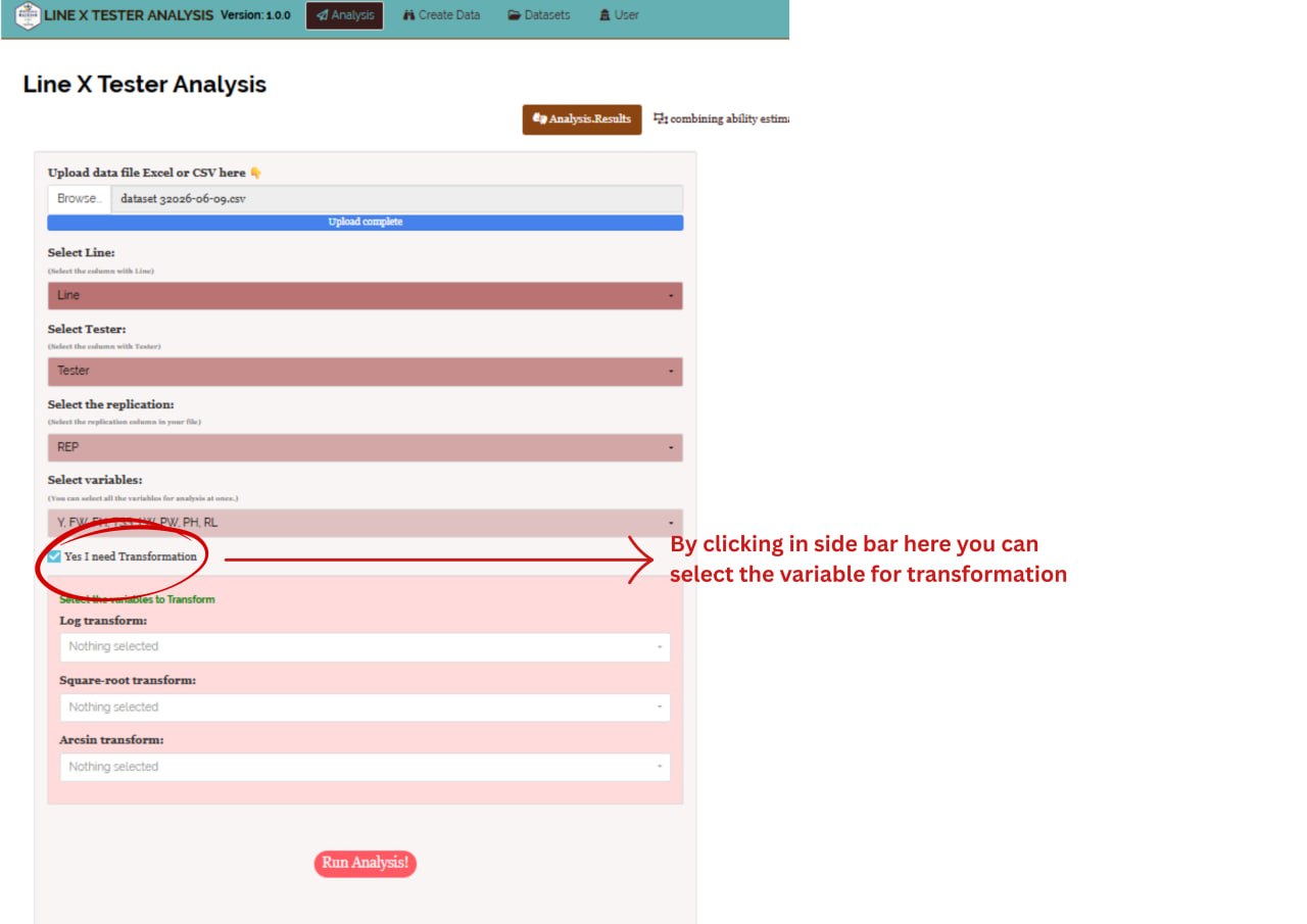
For some data, when there are large number of zeros/ discrete values/ when the observed variables are not normally distributed, we need to do transformation on the dataset (Section 6) . Here, RAISINS provide inbuilt transformation option.
6 Transformation
Log, square root, and arcsine transformations are often used in line x tester analysis to make data more normal and reduce uneven variation. Researchers can use these transformations when analyzing experimental data in RAISINS as shown in Figure 5.
Logarithmic transformation is a mathematical procedure used to convert a skewed distribution into a more symmetrical one by replacing each data point (x) with its logarithm. This technique is specifically applied to positive, continuous data where the variance is proportional to the mean, a relationship common in phenomena that exhibit multiplicative or exponential growth.
Square root transformation is a statistical method used to stabilize variance and reduce right-skewness by replacing each data point (x) with its square root. It is primarily applied to non-negative, discrete “count” data such as those following a Poisson distribution, where the variance of the data tends to increase in proportion to the mean. By compressing the upper end of the scale more significantly than the lower end, this transformation brings the data closer to a normal distribution, satisfying the homoscedasticity requirements of many parametric statistical tests.
Arcsine transformation (also known as the angular transformation) is a mathematical technique specifically designed for data expressed as proportions or percentages bounded between 0 and 1. By taking the inverse sine of the square root of the proportion, this transformation stretches the ends of the distribution near 0 and 1, where variance is naturally small. It is primarily used to achieve homoscedasticity in binomial data.
After choosing the appropriate transformation proceed to Section 7 for analysis.
7 Analysis Results
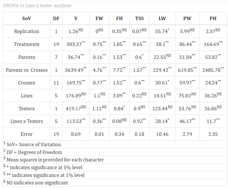
Once your dataset is uploaded and Run Analysis is clicked, the complete Line × Tester ANOVA is performed. The analysis partitions total variation into components due to Crosses (among the p × q hybrids), Lines (GCA of female parents), Testers (GCA of male parents), Line × Tester interaction (SCA), and Error. The F-test for each source of variation determines statistical significance (see Figure 6).
Table 1: ANOVA for Line × Tester Analysis
ANOVA table - sources of variation
The ANOVA for Line × Tester analysis partitions the total sum of squares as follows:
| Source | df | MS | Expected MS |
|---|---|---|---|
| Replications | r−1 | - | - |
| Crosses | pq−1 | MC | σ²e + r·σ²crosses |
| Lines | p−1 | ML | σ²e + rq·σ²GCA(L) |
| Testers | q−1 | MT | σ²e + rp·σ²GCA(T) |
| Lines × Testers | (p−1)(q−1) | MLT | σ²e + r·σ²SCA |
| Error | (pq+p+q)(r−1) | Me | σ²e |
where p = number of lines, q = number of testers, r = number of replications. Significance is indicated by * at 5% and ** at 1% level of probability.
7.1 Interpretation from Figure 6
The ANOVA table reveals significant mean squares due to Treatments, Parents, Parents vs. Crosses, and Crosses for most traits, indicating substantial genetic variability in the experimental material. However, the significance pattern varies considerably across traits and sources of variation. For Lines, mean squares were significant only for Fruit Height (FH) at the 1% level, while Yield (Y), Fruit Weight (FW), TSS, Locule Width (LW), Pericarp Width (PW), and Plant Height (PH) were non-significant, suggesting limited additive genetic diversity among lines for most traits. Testers showed significance only for FH at the 5% level, with all other traits being non-significant. In contrast, the Lines × Testers interaction was highly significant (1% level) for Y, FW, TSS, PW, and PH, and significant at the 5% level for LW, while FH alone was non-significant. This pattern indicates that non-additive (SCA) gene effects predominate over additive (GCA) effects for the majority of traits studied.The significant Line × Tester interaction implies that the performance of a specific cross cannot be predicted solely from the GCA of its parents, making the identification of superior specific cross combinations essential. The error mean squares are consistently low across all traits (ranging from 0.01 for FW to 10.46 for LW), reflecting good experimental precision and validating the reliability of the estimates. These results justify further estimation of GCA and SCA effects and computation of heterosis statistics.
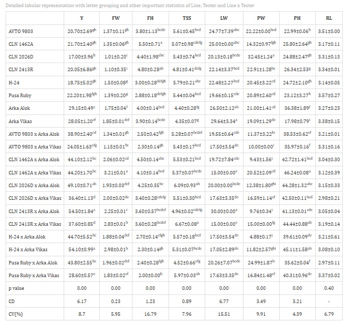
Table 2: Detailed tabular representation with letter grouping and other important statistics of Line, Tester and Line x Tester
8 Multiple comparison tests
What is a Post-hoc test?
-
A post-hoc test is a follow-up analysis performed after finding a significant result in an overall statistical test (like ANOVA or the Line × Tester F-test). Its purpose is to identify exactly which groups or treatments differ from each other. In the context of a Line × Tester analysis, it helps pinpoint where the differences lie among Lines, Testers, and their combinations (hybrids), when the initial F-test shows that not all treatment means are equal.
After obtaining a significant F-value in the Line × Tester ANOVA (for traits such as Y, FW, FH, TSS, LW, PW, and PH in the example), multiple comparison tests are employed to identify which specific treatment means - Lines, Testers, or Line × Tester (hybrid) combinations - differ significantly from one another. Commonly used post-hoc tests include the Least Significant Difference (LSD), Tukey’s Honest Significant Difference (HSD), and Duncan’s Multiple Range Test (DMRT). Each differs in its level of Type I error control and suitability depending on the number of Lines, Testers, and experimental conditions (see Figure 7).
In the Line × Tester framework, the analysis partitions treatment variation into:
- Lines (female parents) - e.g., AVTO 9803, CLN 1462A, CLN 2026D, CLN 2413R, H-24, Pusa Ruby
- Testers (male parents) - e.g., Arka Alok, Arka Vikas
- Line × Tester interaction - representing hybrid-specific (specific combining ability) effects
Post-hoc tests are applied to the treatment means of Lines, Testers, and hybrids for all statistically significant traits identified in the ANOVA summary table. Non-significant traits (e.g., RL in the example) are excluded from further pairwise comparison.
9 Combining Ability Estimates
Combining ability effects are the core output of the Line × Tester analysis. RAISINS automatically estimates GCA effects for each line and tester, and SCA effects for all p × q cross combinations, along with their standard errors and tests of significance (see Figure 8 and Figure 9).
9.1 General Combining Ability (GCA)
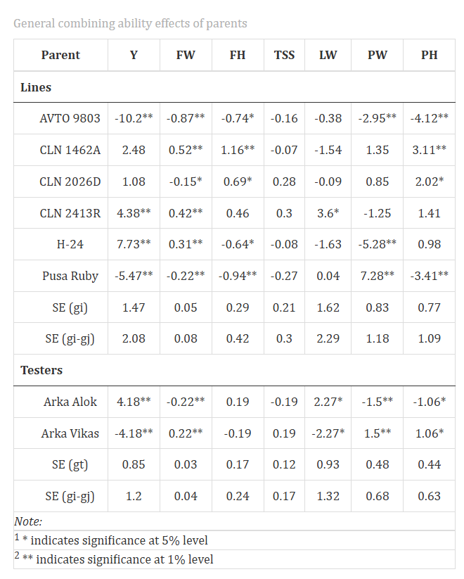
Table 3: GCA effects of lines and testers
GCA - formula and interpretation
The GCA effect of the i-th line is estimated as:
\[\hat{g}_i = \bar{X}_{i..} - \bar{X}_{...}\]
where \(\bar{X}_{i..}\) is the mean of all crosses involving line i and \(\bar{X}_{...}\) is the overall mean of all crosses.
Similarly, the GCA effect of the j-th tester:
\[\hat{g}_j = \bar{X}_{.j.} - \bar{X}_{...}\]
The standard error of a GCA effect for a line:
\[SE(\hat{g}_i) = \sqrt{\frac{M_e}{rq}}\]
For a tester:
\[SE(\hat{g}_j) = \sqrt{\frac{M_e}{rp}}\]
A positive GCA effect indicates that the parent contributes to above-average performance of its progenies, while a negative GCA is desirable for traits where lower values are preferred (e.g., days to maturity). Parents with high positive GCA for target traits are identified as good general combiners and recommended for use in population improvement and as parental lines in hybrid programmes.
9.2 Interpretation from Figure 8
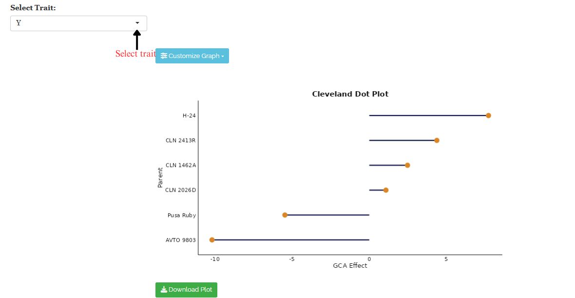
Among the lines, H-24 (7.73**) and CLN 2413R (4.38**) exhibited the highest positive GCA effects for yield, identifying them as good general combiners for this trait. CLN 1462A showed significant positive GCA for Fruit Weight and Fruit Height, while Pusa Ruby had significantly negative GCA for yield and Plant Height. AVTO 9803 recorded significantly negative GCA across most traits, making it a poor general combiner. Among testers, Arka Alok showed significantly positive GCA for yield (4.18**) and Locule Width, whereas Arka Vikas was superior for Fruit Weight and Pericarp Width. Lines and testers with GCA effects significantly different from zero contribute predominantly to additive genetic variance and are prioritised for population improvement programmes and hybrid breeding decisions.
9.3 Specific Combining Ability (SCA)
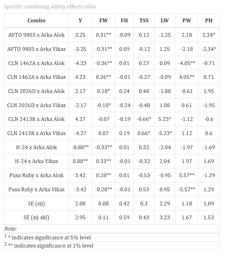
Table 4: SCA effects of all crosses
SCA - formula and interpretation
The SCA effect of the cross between the i-th line and j-th tester is estimated as:
\[\hat{s}_{ij} = \bar{X}_{ij.} - \bar{X}_{i..} - \bar{X}_{.j.} + \bar{X}_{...}\]
where \(\bar{X}_{ij.}\) is the mean of the ij-th cross, \(\bar{X}_{i..}\) is the line mean, \(\bar{X}_{.j.}\) is the tester mean, and \(\bar{X}_{...}\) is the overall mean.
The standard error of an SCA effect:
\[SE(\hat{s}_{ij}) = \sqrt{\frac{(p-1)(q-1)}{pq} \cdot \frac{M_e}{r}}\]
A positive SCA effect for desirable traits indicates that the cross performs better than expected based on the GCA of its parents alone - a manifestation of specific heterosis or favourable non-additive gene action. Crosses with significant and large positive SCA are prioritised as candidates for hybrid variety development.
9.4 Interpretation from Figure 9
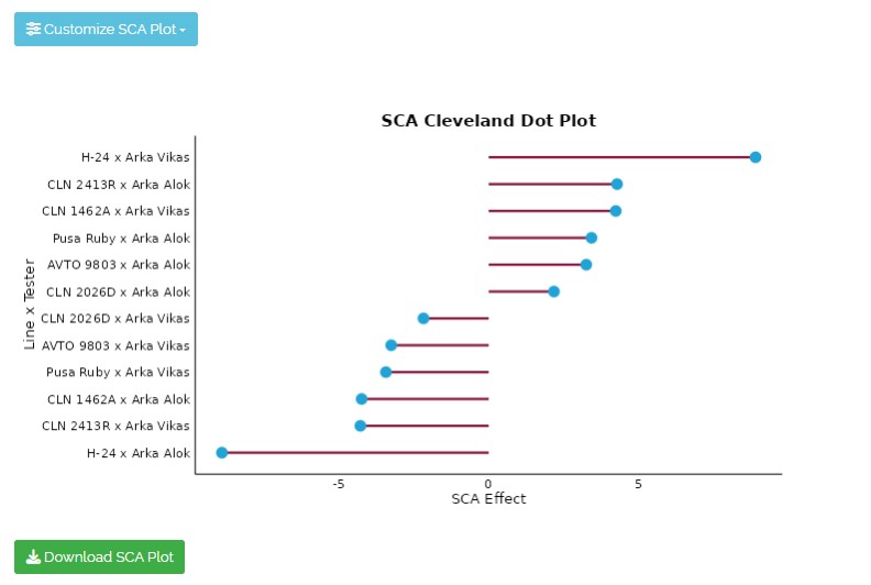
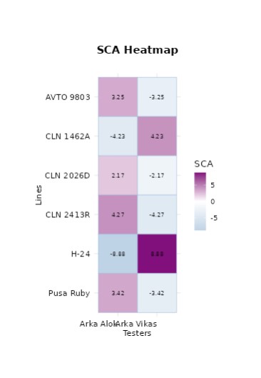
H-24 × Arka Vikas exhibited the highest positive SCA effect for yield (8.88**), making it the most favourable specific combination, while H-24 × Arka Alok showed the largest negative SCA (-8.88**) for the same trait. For Fruit Weight, CLN 1462A × Arka Vikas (0.36**) and AVTO 9803 × Arka Alok (0.31**) were notable positive combiners. Pusa Ruby × Arka Alok showed significantly positive SCA for Pericarp Width (5.57**). Notably, some crosses involving parents with moderate GCA displayed high SCA effects, confirming the predominance of non-additive gene action. Crosses with significantly positive SCA effects, particularly H-24 × Arka Vikas, are strong candidates for commercial hybrid development, while crosses with negative SCA are not recommended for traits where higher values are desirable.
10 % Contribution
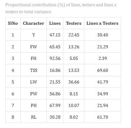
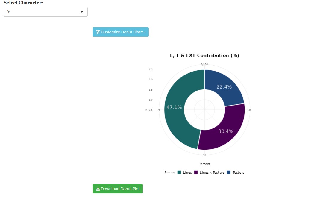
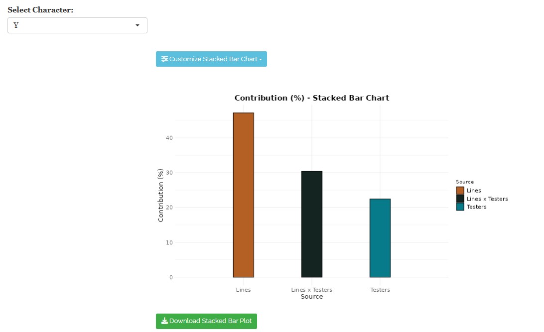
The proportional contribution of Lines, Testers, and Lines × Testers interaction to the total variance is estimated to understand the relative importance of additive and non-additive gene effects across traits. RAISINS presents this as a tabular summary (Figure 13) along with three downloadable visualizations: a Donut Chart (Figure 14), a Stacked Bar Chart (Figure 15), and a Radial Bar Chart (Figure 16).
Table: Proportional contribution (%) of lines, testers, and lines × testers to total variance
% Contribution - formulae and interpretation
The proportional contribution of each source is computed as:
\[\text{Contribution of Lines (\%)} = \frac{SS_{\text{Lines}}}{SS_{\text{Crosses}}} \times 100\]
\[\text{Contribution of Testers (\%)} = \frac{SS_{\text{Testers}}}{SS_{\text{Crosses}}} \times 100\]
\[\text{Contribution of L} \times \text{T (\%)} = \frac{SS_{L \times T}}{SS_{\text{Crosses}}} \times 100\]
A higher contribution of Lines and Testers indicates predominantly additive gene action, while a higher Lines × Testers contribution reflects non-additive gene action governing the trait.
10.1 Interpretation from Figure 13
Lines contributed the most to total variance for Fruit Height (92.56%), Fruit Weight (65.45%), and Plant Height (67.99%), indicating the predominance of additive gene action for these traits. In contrast, Lines × Testers interaction contributed maximally for TSS (69.60%), RL (61.70%), and LW (41.79%), suggesting non-additive gene effects for these characters. For yield, Lines accounted for 47.15%, Lines × Testers for 30.40%, and Testers for 22.45%, indicating a mix of both additive and non-additive effects.
Donut Chart: L, T & LXT Contribution (%) for Yield
Stacked Bar Chart: Contribution (%) for Yield
Radial Bar Chart: Contribution (%) for Yield
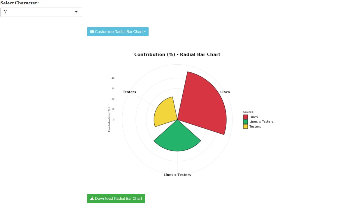
The donut, stacked bar, and radial bar charts for yield visually confirm that Lines (47.1%) contribute the largest share to total genetic variance, followed by Lines × Testers (30.4%) and Testers (22.4%). These charts are customizable and downloadable within RAISINS for reporting purposes.
10.2 Genetic Variance Components
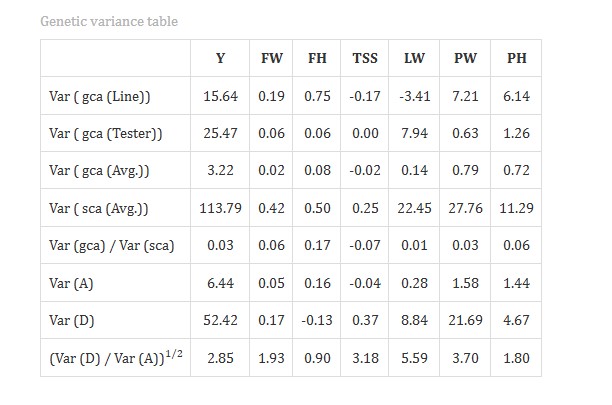
RAISINS estimates genetic variance components including additive variance (Var(A)), dominance variance (Var(D)), GCA variances for lines and testers, and SCA variance, along with the ratio Var(D)/Var(A) to determine the nature of gene action governing each trait ( Figure 17 ).
Table: Genetic variance components
10.3 Interpretation from Figure 17
The dominance variance Var(D) exceeded additive variance Var(A) for most traits, including yield (52.42 vs 6.44), Fruit Weight (0.17 vs 0.05), LW (8.84 vs 0.28), PW (21.69 vs 1.58), and PH (4.67 vs 1.44), confirming the predominance of non-additive gene action. The Var(D)/Var(A) ratio was highest for TSS (3.18) and LW (5.59), further reinforcing dominance effects for these traits. Var(gca)/Var(sca) ratios were consistently below 1.0 across all traits, indicating that SCA effects outweigh GCA effects in governing trait expression.
10.4 Genetic Divergence Parameters & Genetic Advance
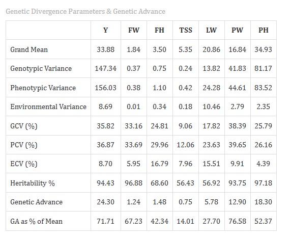
RAISINS estimates key genetic divergence parameters including genotypic and phenotypic variances, heritability, genetic advance, and GCV/PCV for all traits (Figure 18).
Table: Genetic divergence parameters and genetic advance
10.5 Interpretation from Figure 18
High heritability (broad sense) was observed for yield (94.43%), Fruit Weight (96.88%), PW (93.75%), and PH (97.18%), indicating that these traits are largely under genetic control with minimal environmental influence. Genetic Advance as a percentage of mean was highest for yield (71.71%) and PW (76.58%), suggesting that selection would be effective for improving these traits. High heritability coupled with high genetic advance indicates additive gene action and reliable selection response. GCV and PCV values were close for most traits, reflecting low environmental variance and high experimental precision.
11 Heterosis,Heterobeltiosis & standard heterosis
11.1 Heterosis
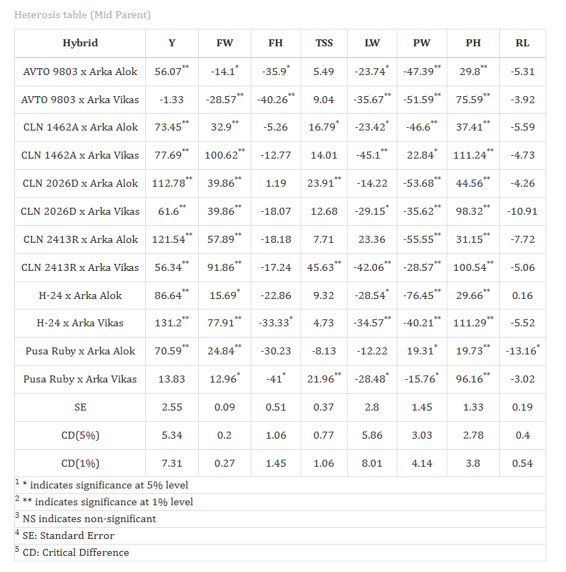
Heterosis refers to the superiority of an F₁ hybrid over its parents and is a key parameter in hybrid breeding. RAISINS computes three types of heterosis for all p × q crosses: Mid-parent Heterosis, Heterobeltiosis (Better-parent Heterosis), and Standard Heterosis (Economic Heterosis) (see Figure 19)
Table 6: Heterosis estimates for all crosses
Heterosis - formulae and interpretation
Mid-parent Heterosis (MPH)
The percentage deviation of the F₁ hybrid mean from the average of its two parents (mid-parent value, MP):
\[MPH (\%) = \frac{\bar{F_1} - MP}{MP} \times 100\]
where \(MP = \frac{P_1 + P_2}{2}\), P₁ = line mean, P₂ = tester mean.
Heterobeltiosis (BPH)
The percentage superiority of the F₁ hybrid over the better parent (BP):
\[BPH (\%) = \frac{\bar{F_1} - BP}{BP} \times 100\]
where BP = max(P₁, P₂) for traits where higher values are desirable (e.g., yield), or min(P₁, P₂) for traits where lower values are desirable (e.g., days to maturity).
Standard Heterosis (SH)
The percentage superiority of the F₁ hybrid over the standard check cultivar (\(\bar{C}\)):
\[SH (\%) = \frac{\bar{F_1} - \bar{C}}{\bar{C}} \times 100\]
Significance of heterosis estimates is tested using the t-test:
\[t = \frac{\text{Heterosis estimate}}{SE(\text{heterosis})}\]
Significant positive values (for yield-related traits) indicate true heterosis. Significance is denoted by * (5%) and ** (1%) as superscripts.
11.2 Interpretation from Figure 19
The heterosis table reveals that the majority of crosses exhibited positive and significant mid-parent heterosis for yield, confirming the presence of genuine hybrid vigour in the experimental material. H-24 × Arka Vikas recorded the highest mid-parent heterosis for yield (131.2**), followed by CLN 2413R × Arka Alok (121.54**) and CLN 2026D × Arka Alok (112.78**), making these the most promising crosses for commercial hybrid development. For Fruit Weight, CLN 1462A × Arka Vikas (100.62**) and CLN 2413R × Arka Vikas (91.86**) showed exceptionally high heterosis. Fruit Height (FH) exhibited predominantly negative mid-parent heterosis across all crosses, which may be desirable depending on the breeding objective. For Pericarp Width, most crosses showed significantly negative heterosis, with H-24 × Arka Alok recording the largest negative value (-76.45**). Crosses with significant positive mid-parent heterosis for yield are strong candidates for further evaluation and commercial hybrid development.
11.3 Heterobeltiosis
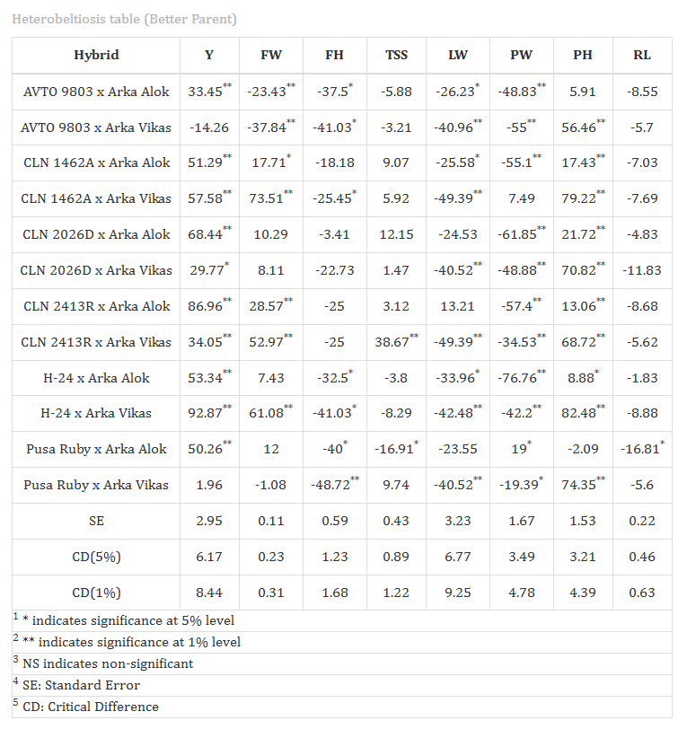
Heterobeltiosis is a more stringent and practically important measure of hybrid vigour than mid-parent heterosis, as it compares the hybrid to the better of its two parents. A cross demonstrating significant positive heterobeltiosis for yield is considered to genuinely outperform both parents and is a priority candidate for commercial hybrid development. RAISINS presents heterobeltiosis estimates alongside their significance levels for all crosses (see Figure 20).
Table 7: Heterobeltiosis estimates
11.4 Interpretation from Figure 20
Among all crosses, H-24 × Arka Vikas (92.87**), CLN 2413R × Arka Alok (86.96**), and CLN 2026D × Arka Alok (68.44**) exhibited the highest significant positive heterobeltiosis for yield, surpassing their better parent in performance and making them priority candidates for multi-location evaluation. For Fruit Weight, CLN 1462A × Arka Vikas (73.51**) and H-24 × Arka Vikas (61.08**) were outstanding. Pericarp Width showed predominantly negative heterobeltiosis across most crosses, with H-24 × Arka Alok (-76.76**) and CLN 2026D × Arka Vikas (-48.88**) recording the largest negative values. For Fruit Height, all crosses exhibited negative heterobeltiosis, which may be desirable depending on the breeding objective. Crosses with non-significant or negative heterobeltiosis for yield are inferior to their better parent and are not recommended for hybrid development.
11.5 Standard Heterosis
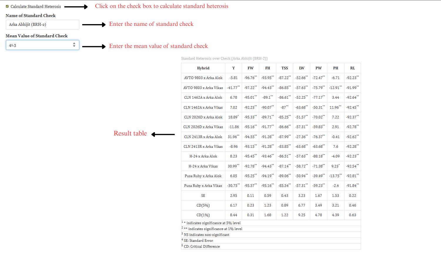
Standard heterosis (economic heterosis) measures the superiority of an F₁ hybrid over a standard commercial check cultivar. It is the most practically relevant form of heterosis from a breeder’s perspective, as it directly indicates the potential of a hybrid to outperform existing commercial varieties. RAISINS computes and presents standard heterosis for all crosses relative to the designated check (see Figure 21).
Table 8u: Standard heterosis estimates relative to the check
11.6 Interpretation from Figure 21
Standard heterosis values greater than zero and statistically significant indicate crosses that outperform the commercial check cultivar Arka Abhijit (BRH-2). For yield, CLN 2413R × Arka Alok (31.96**), H-24 × Arka Vikas (30.99**), and CLN 2026D × Arka Alok (18.89*) showed positive standard heterosis, confirming their superiority over the check. However, the majority of crosses showed strongly negative standard heterosis for Fruit Weight, Fruit Height, TSS, LW, and PW, indicating that the check cultivar Arka Abhijit (BRH-2) performs considerably better for these traits. Pusa Ruby × Arka Vikas recorded the most negative standard heterosis for yield (-30.75**), making it the poorest performer relative to the check. Crosses with significant positive standard heterosis for yield, particularly CLN 2413R × Arka Alok and H-24 × Arka Vikas, are advanced to multi-location trials for varietal release decisions, while crosses falling below check performance are not suitable for commercial deployment.
12 Basic Plots
RAISINS provides a comprehensive suite of publication-ready plots for the Line × Tester analysis. Once Run Analysis is clicked, all relevant plots appear automatically. Navigate to the Basic Plots tab to view them (see Figure 9). Each plot has a gear icon at the top-left corner for customization, and can be downloaded in PNG (300 dpi), JPEG, TIFF, PDF, and SVG formats.
12.1 Customizing Plots
RAISINS provides extensive customization features for all plots. Click on Figure 22 for an overview of the available customization options.
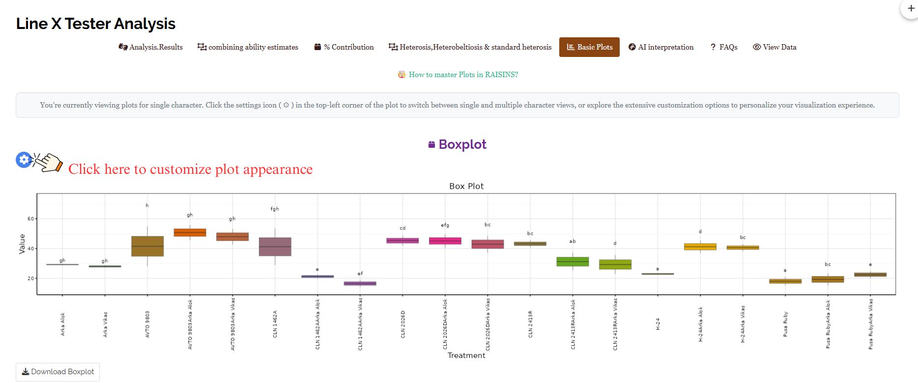
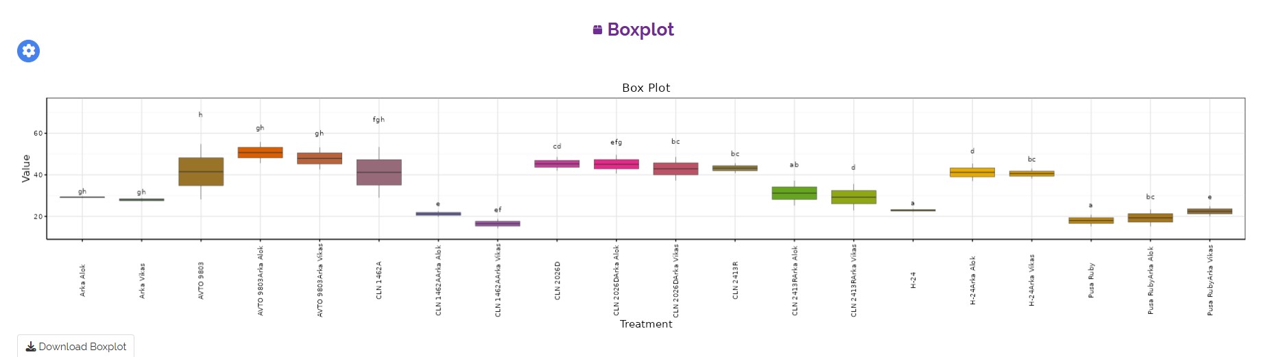
The Boxplot summarises each treatment’s data distribution using the median, interquartile range, and whiskers representing data spread. Colour-coded boxes and compact letter display (CLD) letter groupings indicate statistical differences between treatments. It effectively reveals variability, skewness, and potential outliers within each treatment group, making it well-suited for evaluating consistency and spread of genotype performance across replicated plant breeding or agronomic experiments.
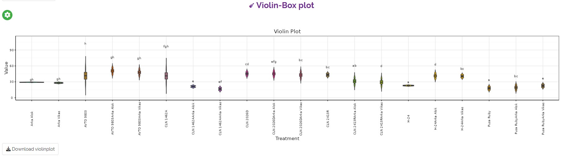
The Violin-Box Plot combines kernel density estimation with embedded boxplot summaries, revealing both distributional shape and key statistics for each treatment. Colour-coded violins and CLD groupings indicate statistical differences between treatments. It simultaneously displays central tendency, variability, and distributional symmetry, making it especially informative in breeding trials where understanding the full spread of replicated observations is critical for evaluating genotypic stability.
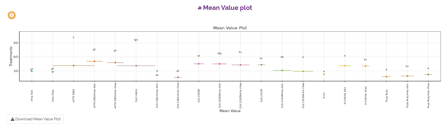
The Mean Value Plot presents treatment means as horizontal points with confidence interval lines in a landscape orientation, facilitating comparison across numerous treatments simultaneously. Colour-coding and CLD groupings convey treatment identity and statistical significance. The horizontal layout minimises visual crowding, clearly displaying both mean magnitude and associated uncertainty, supporting informed selection decisions by highlighting consistently high or low-performing treatments relative to others.
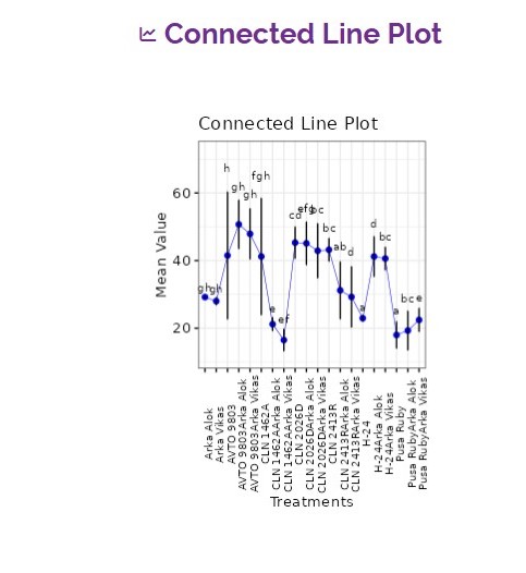
The Connected Line Plot displays treatment means as points linked by a continuous line, with error bars showing standard error. CLD groupings indicate statistical significance between treatments. The connecting line helps visualise trends and deviations across successive treatments, combining the clarity of mean-and-error representation with trend visualisation, making it an effective tool for identifying outstanding or poor-performing treatments in comparative studies.
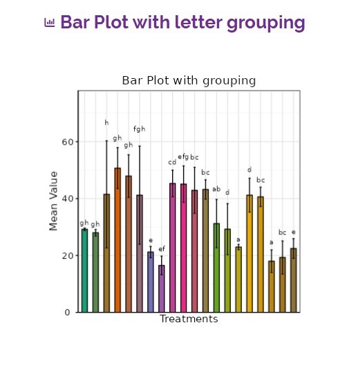
The Bar Plot with Letter Grouping displays treatment means as colour-coded vertical bars with standard error bars. Compact letter display (CLD) notation above each bar indicates statistical significance, where shared letters denote non-significant differences. It enables rapid visual comparison of treatment performance and clearly identifies which treatments differ significantly, making it a valuable tool for summarising ANOVA and post-hoc test results in breeding trials.
13 AI Interpretation
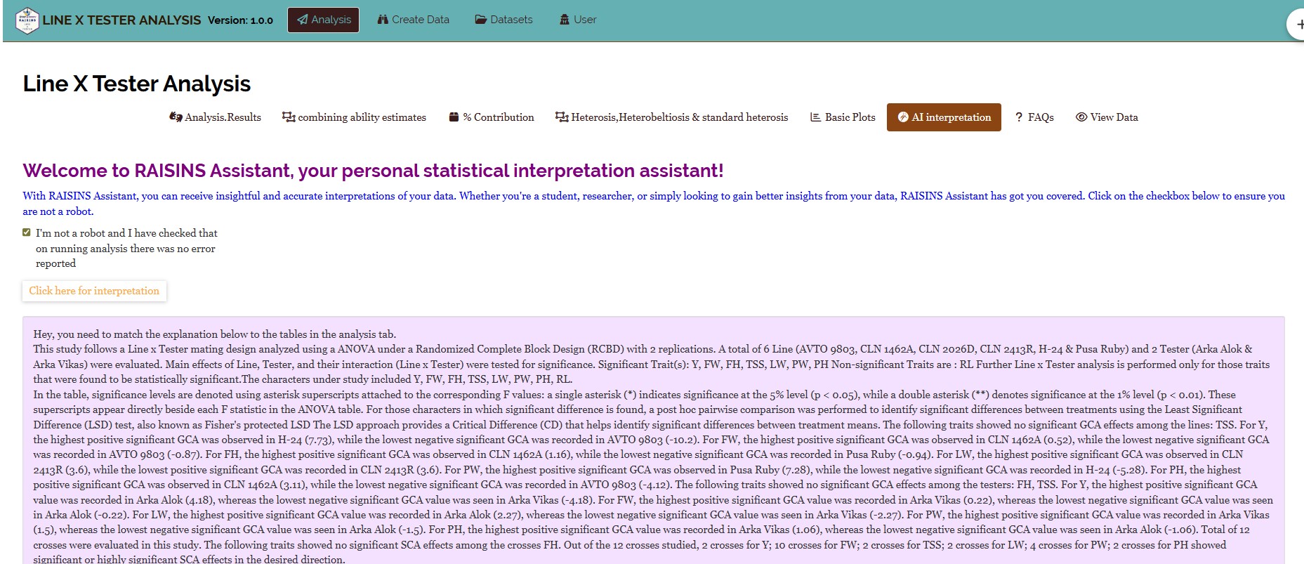
RAISINS is equipped with an AI-powered RAISINS Assistant designed to help users comprehend the outcomes of the Line × Tester analysis. This feature provides clear and concise summaries of combining ability results, identifies statistically significant GCA and SCA effects, and offers informed suggestions for breeding decisions. Click on AI Interpretation in the Analysis tab to generate automated interpretations as shown in Figure 28.
14 Preparing Your Data
“Your analysis is only as good as your data! Feed RAISINS high-quality data, and it will deliver powerful insights - feed it messy data, and the results won’t be trustworthy.”
Create your dataset in MS Excel
Build your dataset directly within the RAISINS app
15 Preparing Data in MS Excel
Open a new blank sheet in MS Excel with only one sheet included. The dataset must follow a column-based format. Include one column each for Line, Tester, and Replication, followed by one column per trait (e.g., Yield, DTF, PH, FW). Each hybrid must appear in a separate row, repeated according to the number of replications. Parents (lines and testers) are also included as separate rows with appropriate labels. The file can be saved in CSV, XLS, or XLSX format; CSV is recommended for faster loading. Ensure no unwanted spaces in column names or genotype names. For reference, see the structure shown in Figure 29.
Dataset Creation Rules
1. Column Naming Convention - No spaces allowed in column names. - Use underscores (_) or full stops (.) for separation. - Avoid symbols and special characters like %, # etc.
- Data Arrangement
- Start data arrangement towards the upper-left corner.
- Ensure the row above the data is not blank.
- Include columns for Line, Tester, Replication, and all trait variables.
- Cell Management
- Avoid typing or deleting in cells without data.
- If needed, select affected cells, right-click, and select Clear Contents.
- Column Relevance
- Name all columns meaningfully.
- Exclude unnecessary columns not required for analysis.
- Parent Entries
- Include all parental lines and testers as separate entries in the dataset.
- Clearly label them to distinguish parents from hybrids.
How to Save as CSV in MS Excel
1. Open Your Workbook - Ensure your data is arranged properly with only one sheet.
- Click ‘File’ Menu
- Go to the top-left corner and click on File.
- Choose ‘Save As’ or ‘Save a Copy’
- Select the location where you want to save your file.
- Set File Type to CSV
- In the ‘Save as type’ dropdown menu, choose CSV (Comma delimited) (*.csv).
- Name Your File
- Enter a relevant file name without spaces (use underscores if needed).
- Click ‘Save’
- Click Save to export the file.
💡 Tip: Before saving, double-check that your data is on the first sheet and follows the required format (no empty rows above the data, meaningful column names, correct assignment of Line, Tester, and Replication columns).
16 Creating Dataset in RAISINS
If you are unsure about the correct format for creating a Line × Tester dataset, RAISINS offers a template-based data creation option directly within the app. Here’s how:
Navigate to the Create Data Tab
Select the number of Lines
Select the number of Testers
Select the number of Replications
Select the number of Traits
Click the Create button
The model layout will appear as shown in Figure 30. Enter observations manually or paste them into the downloaded CSV file. Once data entry is complete, download and upload the CSV file in the Analysis tab.
17 Model Datasets
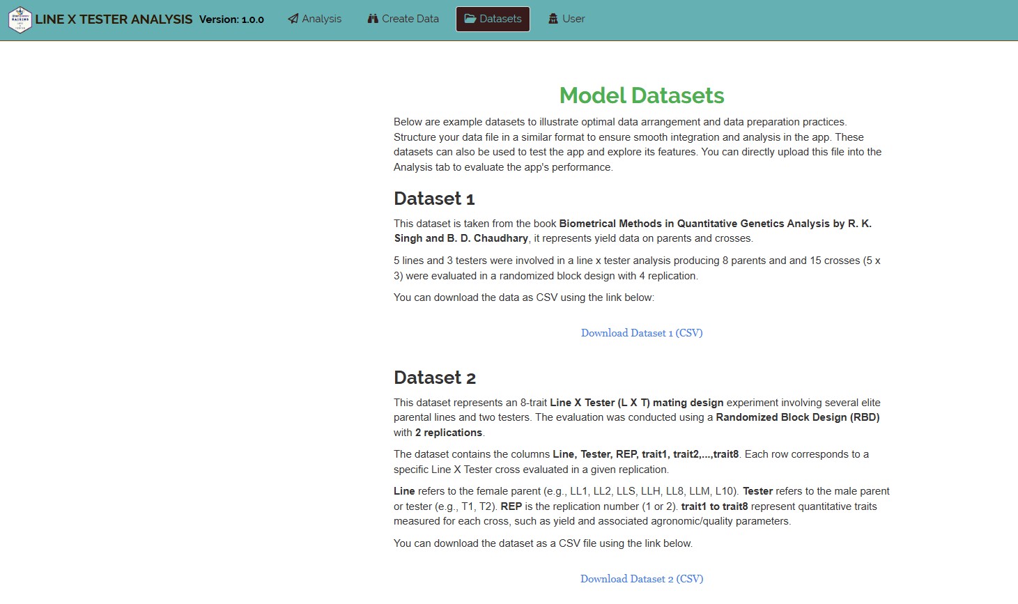
To test the app or better understand the required data arrangement, model datasets are provided within RAISINS. You can download them from the Datasets tab.
18 FAQ’s
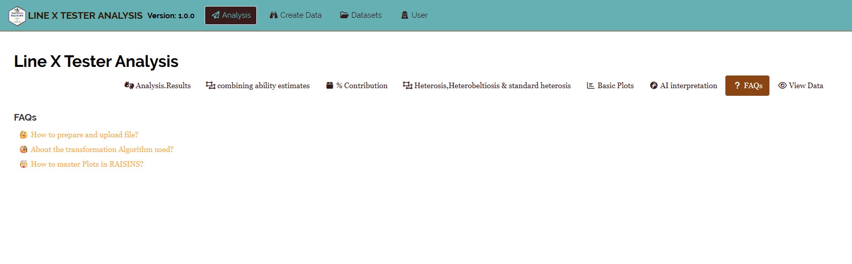
The app includes a dedicated FAQs tab to help clarify common doubts about the Line × Tester analysis and guide users through all features. This section provides detailed answers to frequently asked questions along with helpful tips to ensure a smooth user experience.
19 View Data
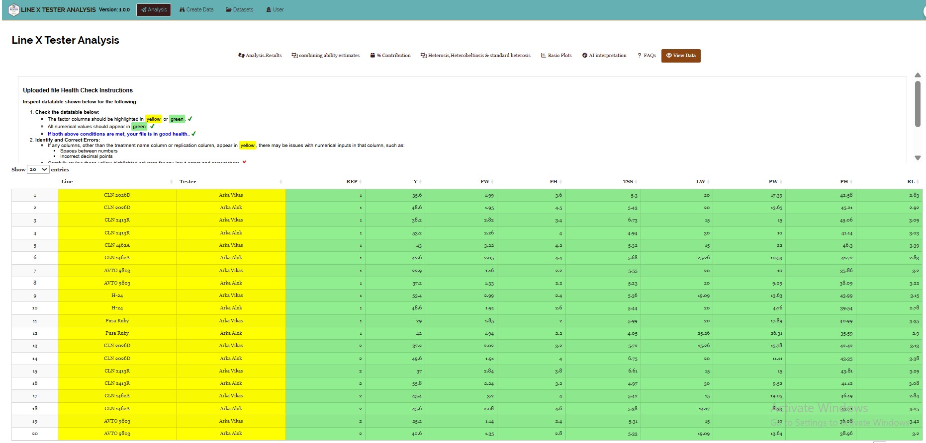
View Data serves as the primary diagnostic tool for ensuring data integrity before analysis. Upon uploading your dataset, the system performs an automated Health Check to validate column types, assignment of Line, Tester, and Replication columns, and overall data formatting. Any detected issues are flagged for correction before proceeding to analysis.