Line × Tester
Line × Tester analysis evaluates the genetic potential of breeding populations. This tutorial explains what combining ability is, how GCA and SCA reveal gene action, and how to run the whole analysis in RAISINS… Read more …
Line × Tester analysis is a widely used mating design in plant breeding for evaluating the combining ability of parental lines and identifying superior hybrid combinations. It partitions genetic variation into General Combining Ability (GCA) and Specific Combining Ability (SCA), helping breeders understand additive and non-additive gene effects. This tutorial begins from first principles: what combining ability actually means, why a good parent and a good hybrid are not the same thing, and how the ANOVA, the variance ratios, and the heterosis estimates fit together into a single breeding decision. It then walks through the complete workflow in RAISINS, including ANOVA tables, GCA and SCA effects, percentage contribution, variance components, genetic parameters, heterosis statistics, publication-ready plots, and AI-assisted interpretation, all without writing a single line of code.
1 What is combining ability?
Suppose you have six promising tomato lines. You want to know which ones to use as parents. The obvious approach is to grow all six, measure their yield, and pick the best two. Reasonable, and often wrong.
Here is the difficulty. A parent’s own performance tells you how that parent behaves. It does not tell you how its children will behave. A tall parent can produce short offspring. A modest-yielding line can throw exceptional hybrids. Breeders learned this the hard way, and the vocabulary they developed for it is combining ability: not how good a parent is, but how good its progeny are.
That single shift raises a second question immediately. When a cross performs well, is it because one parent is reliably good with everybody, or because those two particular parents happen to click with each other? These are different phenomena with different breeding consequences, and Line × Tester analysis exists to tell them apart:
- General Combining Ability (GCA) is a parent’s average performance across all its crosses. A parent with high GCA lifts every hybrid it enters. This is dependable, transmissible, and largely additive.
- Specific Combining Ability (SCA) is what remains for a particular pair after both parents’ GCA has been accounted for. It is the surprise: the cross that does far better, or far worse, than its parents’ track records predict. This is non-additive, arising from dominance and epistasis.
1.1 Why the distinction decides your strategy
This is not a taxonomic exercise. The two kinds of gene action point to two different breeding programmes:
If a trait is governed mainly by additive effects, the good genes pass down predictably. You can select superior parents, intermates them, and the population improves generation after generation. Selection works. Pedigree breeding and population improvement are the right tools.
If a trait is governed mainly by non-additive effects, the advantage lives in the combination, not in the parents, and it will not survive selfing or segregation. You cannot fix it in a pure line. What you can do is identify the specific cross that produces it and sell that F₁ as a hybrid. Hybrid breeding is the right tool.
Choosing wrongly wastes years. This is why the variance ratios in Section 15 matter as much as any single significant p-value.
A little history: Kempthorne, Singh and Chaudhary, and the design itself
-
The Line × Tester mating design was formalised by Kempthorne (1957)
 as a systematic method for evaluating combining ability in crop improvement programmes. It is a practical simplification of the full diallel, in which every parent is crossed with every other parent. A diallel with 20 parents demands 190 crosses, which is rarely feasible in the field. Line × Tester keeps the same logic but restricts the crossing to a set of female parents (lines) against a small set of male parents (testers), so 20 lines against 3 testers needs only 60 crosses while still yielding GCA estimates for every parent and SCA for every combination. The analytical procedure was elaborated by Singh and Chaudhary (1979), whose computational method remains the standard reference in plant breeding.
2 Line x Tester design
The mechanics are simple. You take p lines (female parents) and cross each of them with q testers (male parents), which yields p × q F₁ hybrids. Those hybrids, together with their parents, are then grown in a replicated experiment, usually a Randomised Complete Block Design (RCBD), and every trait of interest is measured. Figure 1 shows the structure for the 6 × 2 example used throughout this tutorial.
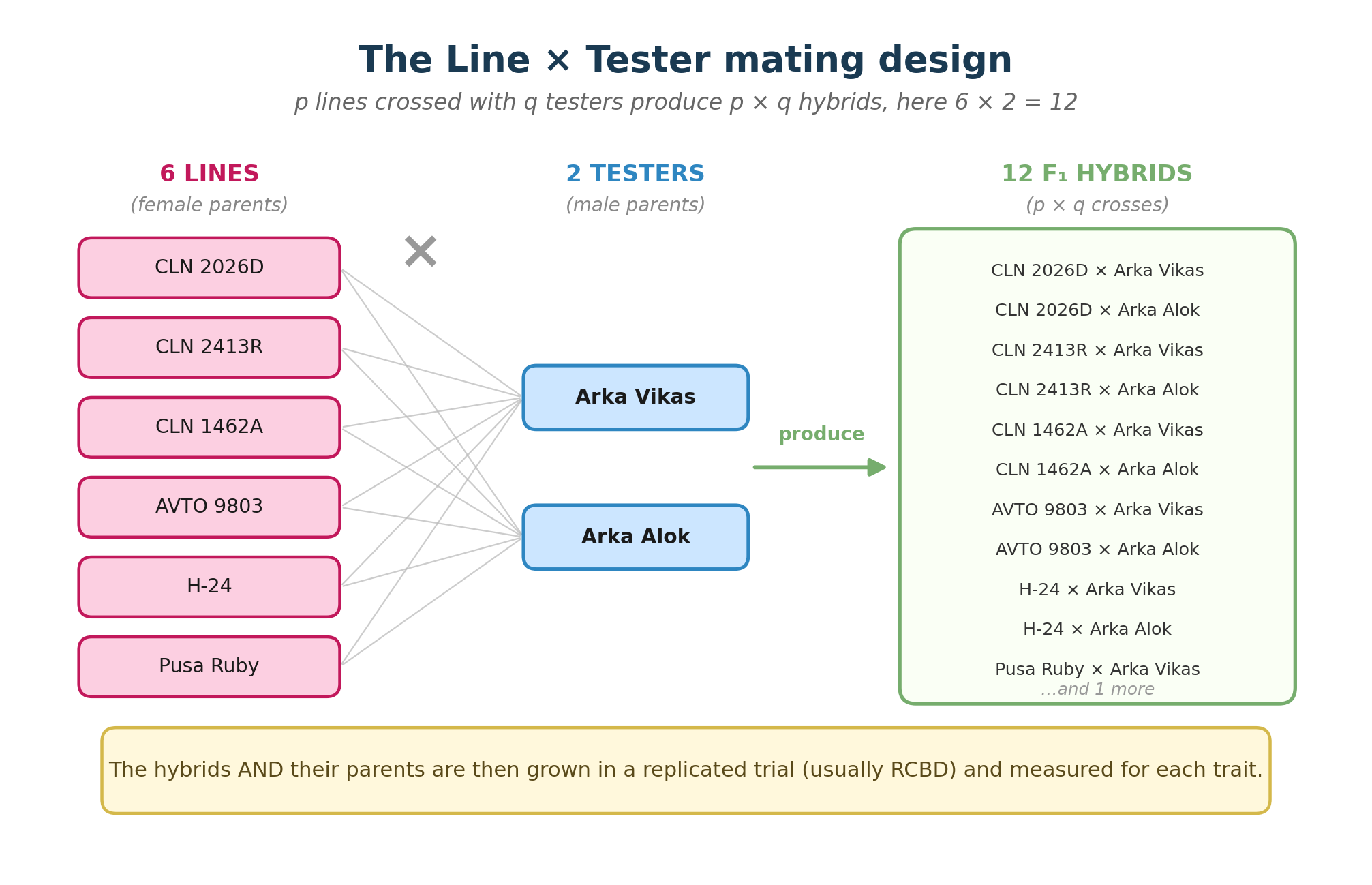
| Term | Meaning | In the example |
|---|---|---|
| Line | Female parent, usually the larger set | 6 lines (CLN 2026D, CLN 2413R, CLN 1462A, AVTO 9803, H-24, Pusa Ruby) |
| Tester | Male parent, usually a small set of well-characterised genotypes | 2 testers (Arka Vikas, Arka Alok) |
| Hybrid (F₁) | The progeny of one line crossed with one tester | 6 × 2 = 12 hybrids |
| Check | A commercial cultivar included for comparison | Arka Abhijit (BRH-2) |
3 How to read the output
Line × Tester produces a great many tables, and newcomers often read them in the wrong order and reach the wrong conclusion. The logic runs in one direction, and it is worth fixing in mind before you look at a single number.
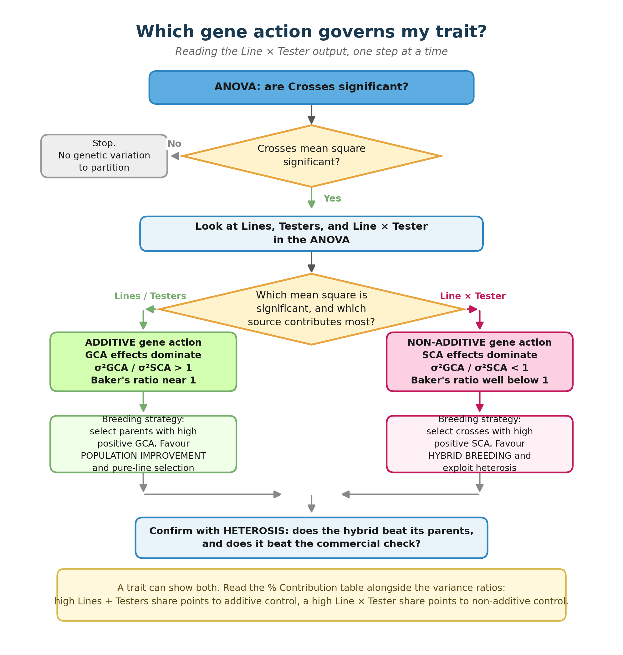
Start with the ANOVA. If Crosses are not significant, there is no genetic variation among your hybrids and nothing further to partition. If Crosses are significant, the analysis splits that variation three ways:
- Lines and Testers mean squares test whether parents differ in their average contribution. Significance here means GCA matters, which means additive gene action.
- The Line × Tester interaction mean square tests whether particular combinations deviate from what their parents’ averages predict. Significance here means SCA matters, which means non-additive gene action.
Then confirm what the ANOVA suggests using the variance ratios and the % contribution table, and finally check the practical payoff with heterosis. Figure 2 shows the whole path.
Baker's ratio and the σ²GCA / σ²SCA ratio
Two summary numbers condense the gene action question.
The σ²GCA / σ²SCA ratio compares the variance due to general combining ability against that due to specific combining ability. A value above 1 indicates additive effects predominate; below 1, non-additive effects predominate.
Baker’s ratio (Baker, 1978) expresses the same idea on a bounded scale:
\[\text{Baker's ratio} = \frac{2\sigma^2_{GCA}}{2\sigma^2_{GCA} + \sigma^2_{SCA}}\]
It runs from 0 to 1. A value approaching 1 means the progeny performance is almost entirely predictable from the parents’ GCA, so selection on parents will work. A value near 0 means GCA tells you almost nothing about which cross will win, so hybrids must be evaluated individually and heterosis exploited directly.
The practical reading: Baker’s ratio close to 1, select parents. Baker’s ratio close to 0, select crosses.
A parent with excellent per se performance is not necessarily a good combiner, and a parent with unremarkable performance can be an excellent one. Never substitute a parent’s own trial mean for its GCA. The whole point of the design is that these two things come apart, and the example in Section 13.1 shows exactly that happening.
4 Assumptions
Like any ANOVA-based method, Line × Tester analysis buys its conclusions on credit. The terms of the loan:
| Assumption | What it means | What if it fails? |
|---|---|---|
| Randomisation | Genotypes assigned to plots at random within each block | Serious. Settled at the design stage, not fixable in analysis |
| Independence | Each plot’s performance is unaffected by its neighbours | Serious. Handled by good field layout and adequate borders |
| Normality | Errors are approximately normally distributed | Try a transformation (Section 10) |
| Homogeneity of variance | Error variance is similar across genotypes and blocks | Try a transformation; consider dropping badly behaved traits |
| Additivity of effects | Block and genotype effects add rather than multiply | Transformation often resolves this |
| No epistasis (for the genetic model) | The GCA/SCA partition assumes digenic effects only | Estimates become approximations; interpret variance ratios cautiously |
The statistical assumptions are the familiar RCBD ones, and RAISINS gives you transformation tools for the two that commonly fail. The genetic assumptions are stronger and rarely hold perfectly in practice, which is why breeders treat GCA and SCA estimates as guides to a decision rather than exact quantities, and confirm promising crosses in multi-location trials before release.
5 Getting to the module
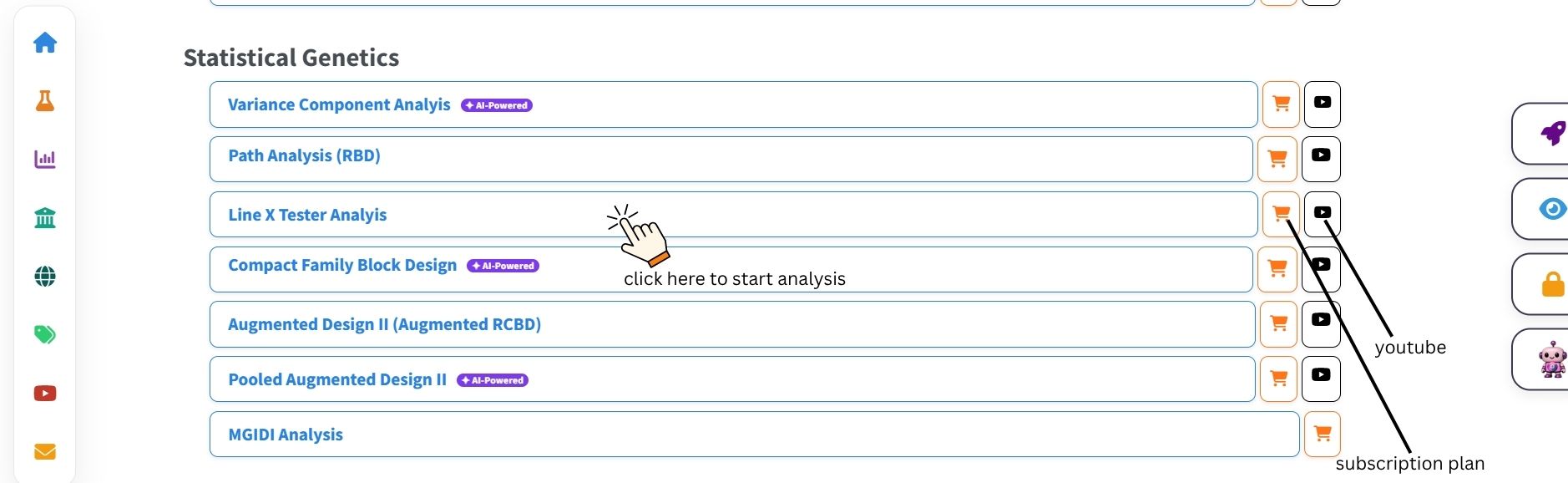
Now that the theory is clear, let us run the analysis. Visit the RAISINS home page at www.raisins.live and go to Statistical Genetics, where the available mating design analyses are listed. In this tutorial we use the Line × Tester module, shown in Figure 3.
5.1 Computational Provenance & Reproducibility Record
CPRR (Computational Provenance & Reproducibility Record) provides a transparent and comprehensive record. Click on the icon shown in Figure 3 to access CPRR and know about the computational workflow performed during the analysis. The record for this module states the R version and the exact version of every package used, names the specific function behind each reported result. CPRR lists every default parameter and decision rule applied by the module and provides fully runnable R code that reproduces each analytical step. Users can execute the code in R to independently reproduce and verify the results. It carries its own DOI.
To cite the platform itself in a paper, thesis, or report, use the RAISINS citation, available in APA, Harvard, and BibTeX formats at www.raisins.live/citation.html. That is the primary reference, and for most manuscripts it is all you need.
The CPRR for Line × Tester is at www.raisins.live/module_record/linetester.html.
Cite the RAISINS paper as your primary reference for the platform. Add the CPRR as supporting documentation when a journal asks for details of the computing environment, or when you want your methods section to be precise about versions and functions rather than saying “analysis was carried out using an online tool.” The CPRR supports the citation and ensures computational reproducibility.
6 Preview mode and Quick Tour
Before subscribing, you can explore the entire module using Preview mode, accessible from the Welcome page. Preview mode loads built-in datasets so you can try every feature (ANOVA, combining ability estimates, heterosis, plots, and the RA-One assistant) without uploading your own data. First-time users are also offered a Quick Tour, an interactive, step-by-step walkthrough that highlights each control and explains what it does. You can retake the tour at any time from the Quick Tour tab.
7 A working example
To keep things concrete, the whole tutorial follows one experiment. Six lines (CLN 2026D, CLN 2413R, CLN 1462A, AVTO 9803, H-24, and Pusa Ruby) were crossed with two testers (Arka Vikas and Arka Alok) to produce 12 F₁ hybrids. The hybrids and their parents were evaluated in an RCBD with two replications, and observations were recorded for eight quantitative traits: Yield (Y), Fruit Weight (FW), Fruit Height (FH), Total Soluble Solids (TSS), Locule Width (LW), Pericarp Width (PW), Plant Height (PH), and Rind Length (RL).
The aim is to estimate combining ability, identify good general and specific combiners, determine the nature of gene action for each trait, and compute heterosis for each cross. The dataset structure is shown in Figure 4.
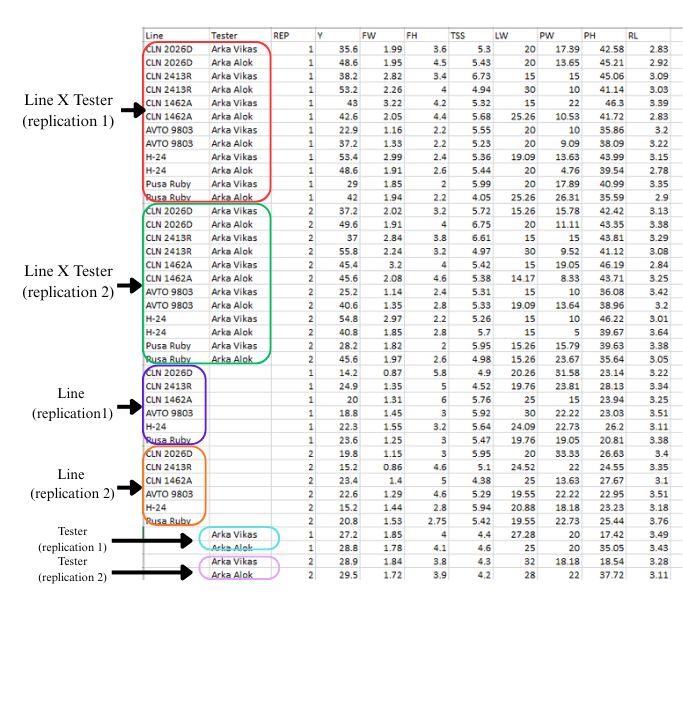
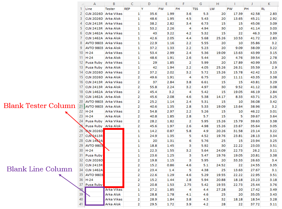
When entering parents, leave the opposite parent cell completely empty. Do not enter NA, dots (.), hyphens (-), zeros, spaces, or any placeholder symbol. RAISINS uses emptiness itself to recognise a row as a parent rather than a hybrid, and any character in that cell will be read as a genotype name (Figure 5).
8 How to prepare your data
Your analysis is only as good as your data. Feed RAISINS high-quality data and it will deliver powerful insights; feed it messy data and the results will not be trustworthy. You have four routes:
- Create your dataset in MS Excel
- Build your dataset directly within the RAISINS app
- Use the model datasets in RAISINS as a reference
- Create your dataset using the RA-One chat assistant
8.1 Preparing data in MS Excel
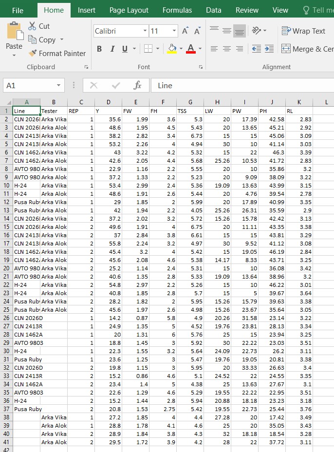
Open a new blank sheet in MS Excel containing only one sheet, and avoid adding any unnecessary content. The dataset follows a column-based format: one column each for Line, Tester, and Replication, followed by one column per trait (e.g. Yield, FW, FH, TSS). Each hybrid appears in a separate row, repeated according to the number of replications, and the parents appear as their own rows with the opposite parent cell left empty. The file can be saved as CSV, XLS, or XLSX, but CSV is recommended as it is lighter and loads faster. Ensure there are no unwanted spaces in column names or genotype names. For reference, see the structure in Figure 6.
Dataset creation rules
- Column naming convention
- No spaces allowed in column names.
- Use underscores (
_) or full stops (.) for separation. - Avoid symbols and special characters such as %, #.
- Data arrangement
- Start the data towards the upper-left corner, from cell A1.
- Ensure the row above the data is not blank.
- Include columns for Line, Tester, Replication, and all trait variables.
- Column 1 holds the lines, repeated according to testers and replications. Column 2 holds the testers, repeated according to lines and replications. Column 3 holds the replications. Traits follow from column 4 onwards.
- Cell management
- Avoid typing or deleting in cells without data.
- If needed, select the affected cells, right-click, and choose Clear Contents.
- Column relevance
- Name all columns meaningfully.
- Exclude unnecessary columns not required for the analysis.
- Parent entries
- Include all parental lines and testers as separate rows.
- Leave the opposite parent cell completely empty so parents are distinguished from hybrids.
- Keep spelling and capitalisation of genotype names consistent throughout.
How to save as CSV in MS Excel
Open your workbook. Ensure your data is arranged properly with only one sheet.
Click the ‘File’ menu. Go to the top-left corner and click File.
Choose ‘Save As’ or ‘Save a Copy’. Select the location where you want to save your file.
Set file type to CSV. In the ‘Save as type’ dropdown, choose CSV (Comma delimited) (*.csv).
Name your file. Enter a relevant file name without spaces (use underscores if needed).
Click ‘Save’. Click Save to export the file.
💡 Tip: Before saving, double-check that your data is on the first sheet and follows the required format: no empty rows above the data, meaningful column names, correct assignment of Line, Tester, and Replication columns, and empty cells in the opposite parent column for parent rows.
If you have any doubt about saving a file as CSV or about the basics of data preparation, see our getting started tutorial here.
8.2 Creating a dataset in RAISINS
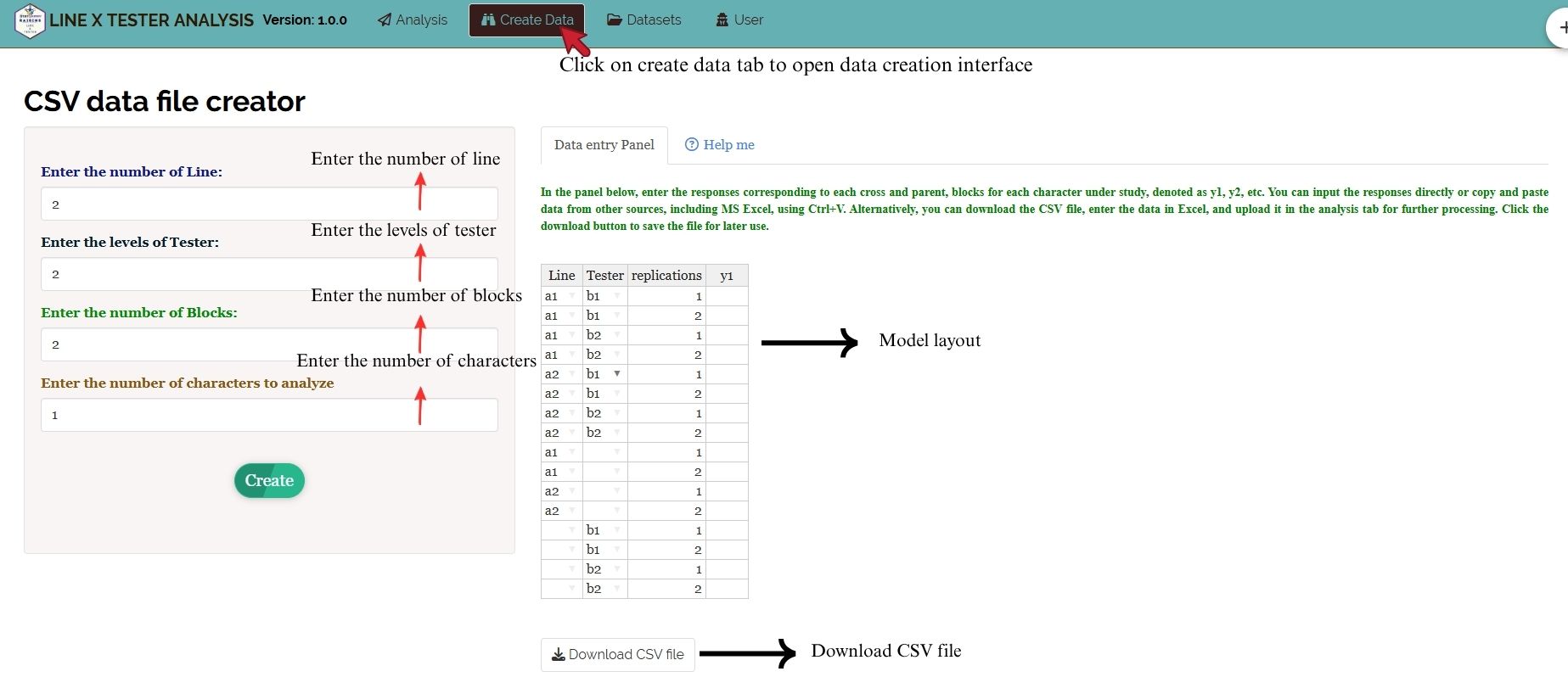
If you are unsure about the correct format, RAISINS can create the layout for you using the prescribed template. Here is how:
- Navigate to the Create Data tab
- Select the number of Lines
- Select the number of Testers
- Select the number of Replications
- Select the number of Traits
- Click the Create button
The model layout appears as shown in Figure 7. You may enter the observations manually into the template or paste them from an existing Excel file. Once data entry is complete, download the CSV and upload it under the Analysis tab.
8.3 Model datasets
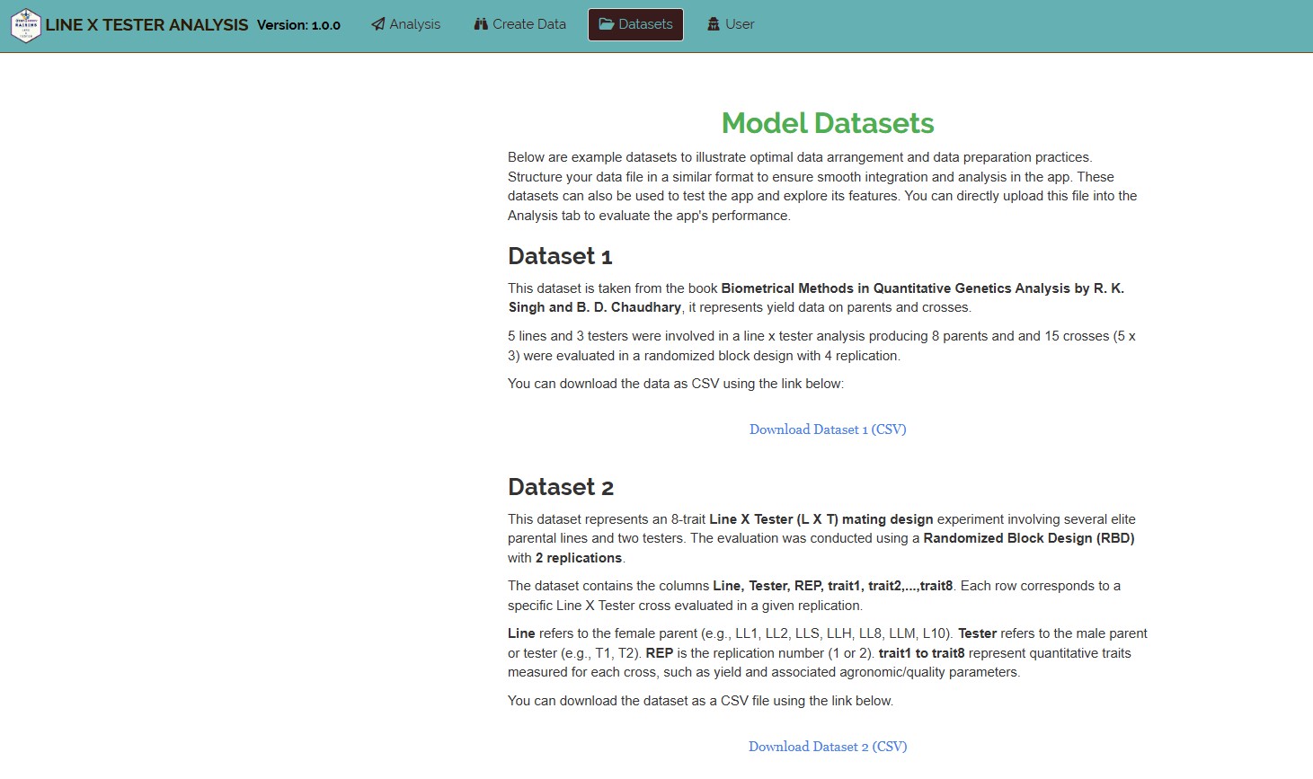
To test the module or to better understand the data arrangement, model datasets are provided within the app. You can download them from the Datasets tab.
9 The Analysis tab
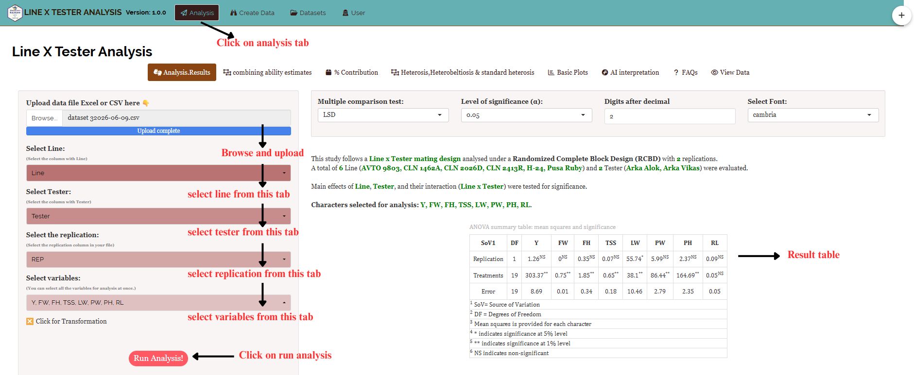
Figure 9 shows the Analysis tab in detail, with each option explained. Upload your prepared file by clicking Browse in the sidebar. Once uploaded, selectors appear for assigning the Lines, Testers, Replication, and trait Variables columns. Click Run Analysis and all outputs appear instantly across the sub-tabs.
If a trait contains many zeros or discrete values, or is not normally distributed, apply a transformation first (Section 10).
10 Transformation
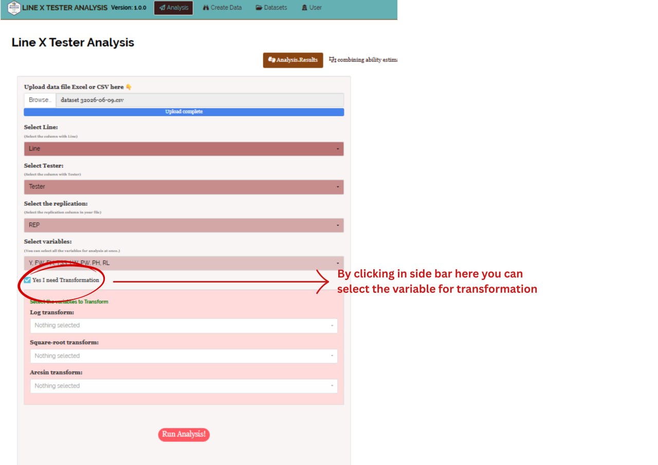
Log, square root, and arcsine transformations are used to make data more normal and to even out uneven variation. You can apply them directly in RAISINS as shown in Figure 10.
Logarithmic transformation converts a skewed distribution into a more symmetrical one by replacing each data point (x) with its logarithm. It is applied to positive, continuous data where the variance grows in proportion to the mean, a pattern common in phenomena that grow multiplicatively or exponentially.
Square root transformation stabilises variance and reduces right-skewness by replacing each data point (x) with its square root. It is primarily used for non-negative count data, such as those following a Poisson distribution, where variance increases with the mean. By compressing the upper end of the scale more than the lower end, it brings the data closer to normality.
Arcsine transformation (the angular transformation) is designed for proportions or percentages bounded between 0 and 1. By taking the inverse sine of the square root of the proportion, it stretches the ends of the distribution near 0 and 1, where variance is naturally small. It is chiefly used to achieve homoscedasticity in binomial data.
After choosing the appropriate transformation, proceed to Section 11 for the analysis.
11 Analysis results
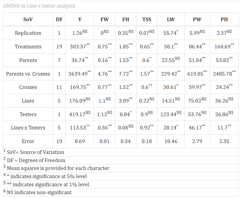
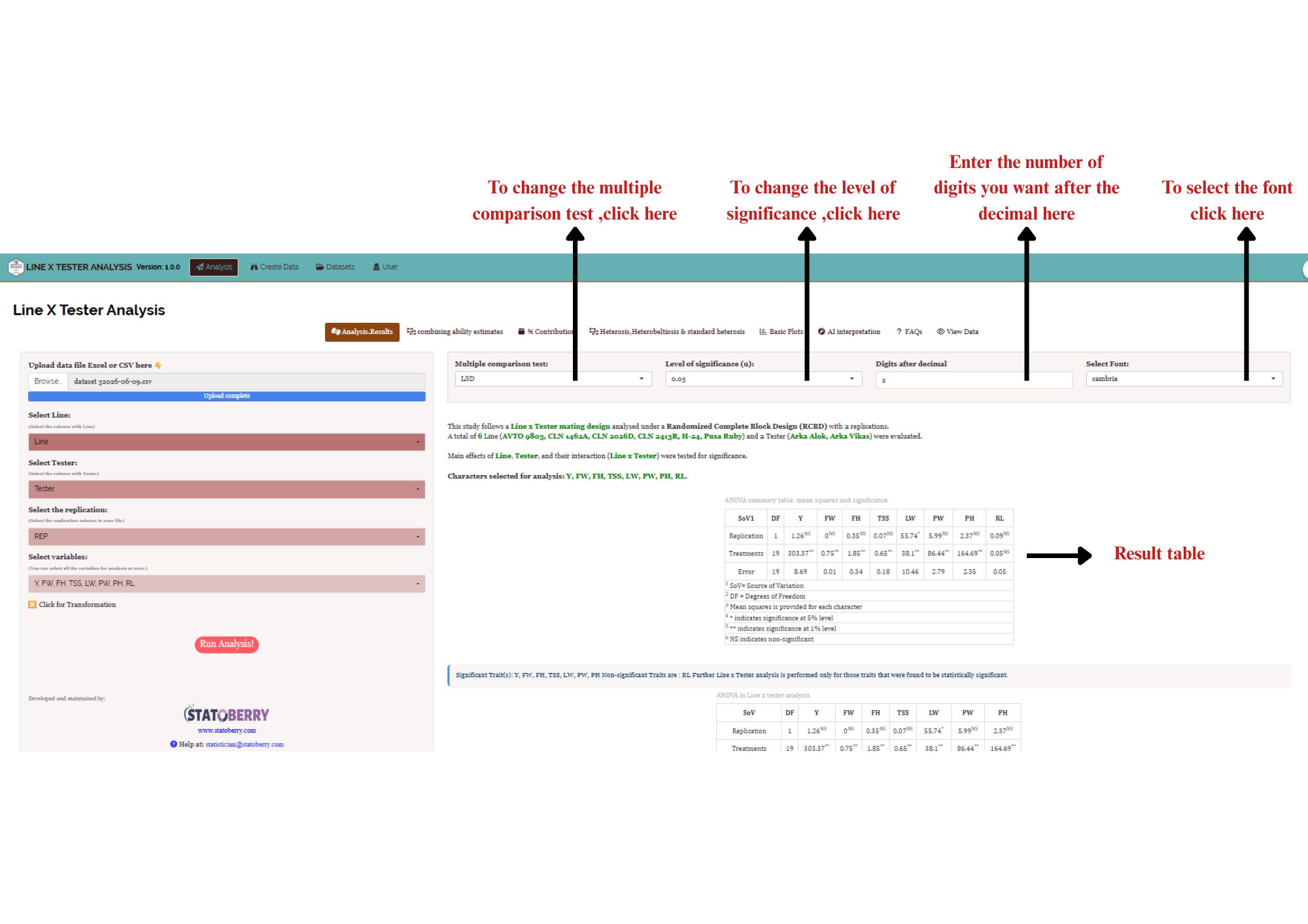
Once your dataset is uploaded and you click Run Analysis, the complete Line × Tester ANOVA is performed. The analysis partitions total variation into components due to Crosses (among the p × q hybrids), Lines (GCA of female parents), Testers (GCA of male parents), the Line × Tester interaction (SCA), and Error. An F-test on each source determines significance (Figure 11).
Table 1: ANOVA for Line × Tester analysis
ANOVA table: sources of variation
The ANOVA for Line × Tester analysis partitions the total sum of squares as follows:
| Source | df | MS | Expected MS |
|---|---|---|---|
| Replications | r−1 | - | - |
| Crosses | pq−1 | MC | σ²e + r·σ²crosses |
| Lines | p−1 | ML | σ²e + rq·σ²GCA(L) |
| Testers | q−1 | MT | σ²e + rp·σ²GCA(T) |
| Lines × Testers | (p−1)(q−1) | MLT | σ²e + r·σ²SCA |
| Error | (pq+p+q)(r−1) | Me | σ²e |
where p = number of lines, q = number of testers, r = number of replications. Significance is indicated by * at the 5% and ** at the 1% level of probability.
Reading the Expected MS column tells you why each F-test works: the Lines mean square carries σ²GCA(L) in addition to error, so testing ML against Me isolates the line GCA component. The same logic applies to Testers and to the interaction.
Interpretation from Figure 11
The ANOVA shows significant mean squares for Treatments, Parents, Parents vs. Crosses, and Crosses for most traits, indicating substantial genetic variability in the experimental material. The pattern beneath that headline is where the interest lies.
For Lines, mean squares were significant only for Fruit Height at the 1% level; Yield, Fruit Weight, TSS, Locule Width, Pericarp Width, and Plant Height were non-significant, suggesting limited additive diversity among lines for most traits. Testers showed significance only for Fruit Height at the 5% level. In contrast, the Lines × Testers interaction was highly significant (1%) for Yield, Fruit Weight, TSS, Pericarp Width, and Plant Height, and significant at 5% for Locule Width, with Fruit Height alone non-significant.
Read against Section 3, this pattern says something specific: non-additive (SCA) effects predominate over additive (GCA) effects for most traits studied. The significant interaction means the performance of a given cross cannot be predicted from its parents’ GCA alone, so identifying superior specific combinations becomes essential. Error mean squares are consistently low across traits (0.01 for FW up to 10.46 for LW), reflecting good experimental precision and validating the estimates that follow.
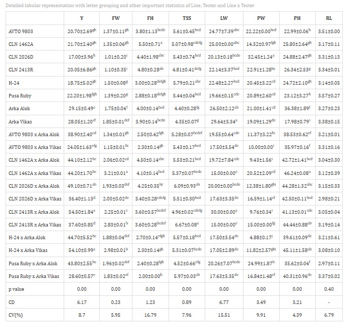
Table 2: Detailed representation with letter grouping and other statistics
12 Multiple comparison tests
What is a post-hoc test?
-
A post-hoc test is a follow-up analysis performed after finding a significant result in an overall statistical test such as ANOVA or the Line × Tester F-test. The F-test tells you that some means differ, but not which ones. A post-hoc test identifies exactly where the differences lie among Lines, Testers, and their hybrid combinations.
After a significant F-value in the Line × Tester ANOVA, multiple comparison tests identify which specific treatment means differ from one another. RAISINS offers the Least Significant Difference (LSD) test and Tukey’s Honest Significant Difference (HSD) test. They differ in how strictly they control Type I error, and the right choice depends on the number of genotypes and the purpose of the comparison (Figure 12).
Post-hoc tests are applied to the treatment means of Lines, Testers, and hybrids for all statistically significant traits identified in the ANOVA. Non-significant traits (Rind Length in this example) are excluded from pairwise comparison, since the F-test has already found no differences worth locating.
13 Combining ability estimates
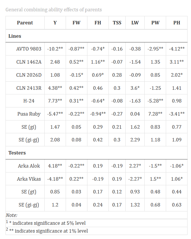
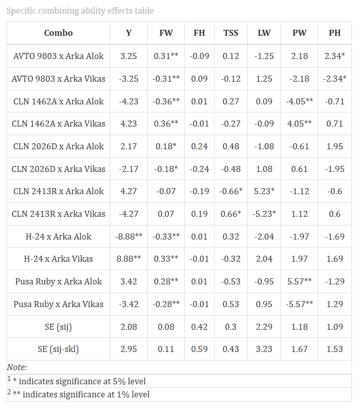
Combining ability effects are the core output of the analysis. RAISINS estimates GCA effects for every line and tester, and SCA effects for all p × q cross combinations, with standard errors and tests of significance (Figure 13 and Figure 14).
13.1 General Combining Ability (GCA)
Table 3: GCA effects of lines and testers
GCA: formula and interpretation
The GCA effect of the i-th line is estimated as:
\[\hat{g}_i = \bar{X}_{i..} - \bar{X}_{...}\]
where \(\bar{X}_{i..}\) is the mean of all crosses involving line i and \(\bar{X}_{...}\) is the overall mean of all crosses. Notice what this says: a line’s GCA is simply how far its progeny average sits from the grand average. Nothing about the line’s own performance enters the formula.
Similarly, the GCA effect of the j-th tester:
\[\hat{g}_j = \bar{X}_{.j.} - \bar{X}_{...}\]
The standard error of a GCA effect for a line:
\[SE(\hat{g}_i) = \sqrt{\frac{M_e}{rq}}\]
For a tester:
\[SE(\hat{g}_j) = \sqrt{\frac{M_e}{rp}}\]
A positive GCA indicates the parent contributes to above-average performance in its progenies. A negative GCA is desirable for traits where lower values are preferred, such as days to maturity or plant height in a lodging-prone crop. Parents with high positive GCA for target traits are good general combiners, recommended for population improvement and as parental lines in hybrid programmes.
Interpretation from Figure 13
Among the lines, H-24 (7.73**) and CLN 2413R (4.38**) showed the highest positive GCA for yield, identifying them as good general combiners. CLN 1462A showed significant positive GCA for Fruit Weight and Fruit Height, while Pusa Ruby had significantly negative GCA for yield and Plant Height. AVTO 9803 recorded significantly negative GCA across most traits, making it a poor general combiner.
Among testers, Arka Alok showed significantly positive GCA for yield (4.18**) and Locule Width, whereas Arka Vikas was superior for Fruit Weight and Pericarp Width. Note that the two testers are not interchangeable: which one you should use depends on the trait you are breeding for.
Lines and testers with GCA significantly different from zero contribute predominantly to additive variance and are prioritised for population improvement.
13.2 Specific Combining Ability (SCA)
Table 4: SCA effects of all crosses
SCA: formula and interpretation
The SCA effect of the cross between the i-th line and j-th tester is estimated as:
\[\hat{s}_{ij} = \bar{X}_{ij.} - \bar{X}_{i..} - \bar{X}_{.j.} + \bar{X}_{...}\]
where \(\bar{X}_{ij.}\) is the mean of the ij-th cross, \(\bar{X}_{i..}\) is the line mean, \(\bar{X}_{.j.}\) is the tester mean, and \(\bar{X}_{...}\) is the overall mean.
The formula is worth reading slowly, because it is the whole idea of SCA in one line. Take the cross’s actual performance, subtract what the line’s GCA led you to expect, subtract what the tester’s GCA led you to expect, then add back the grand mean (which you have now subtracted twice). What is left is the part of the cross’s performance that neither parent’s average could predict. That residual is the specific combination.
The standard error of an SCA effect:
\[SE(\hat{s}_{ij}) = \sqrt{\frac{(p-1)(q-1)}{pq} \cdot \frac{M_e}{r}}\]
A positive SCA for a desirable trait indicates the cross performs better than its parents’ GCA alone would suggest, a manifestation of specific heterosis or favourable non-additive gene action. Crosses with large, significant, positive SCA are prioritised for hybrid variety development.
Interpretation from Figure 14
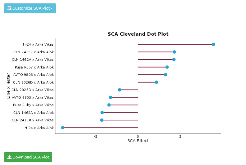
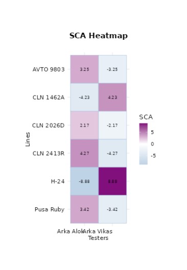
H-24 × Arka Vikas showed the highest positive SCA for yield (8.88**), making it the most favourable specific combination, while H-24 × Arka Alok showed the largest negative SCA (−8.88**) for the same trait. That contrast is instructive: the same line, H-24, produces the best and the worst specific combination depending on which tester it meets. Its high GCA (7.73**) tells you it is a reliable parent on average, and tells you nothing at all about which of its two crosses to pursue. This is precisely the situation Section 1 described, visible in your own numbers.
For Fruit Weight, CLN 1462A × Arka Vikas (0.36**) and AVTO 9803 × Arka Alok (0.31**) were notable positive combiners; the latter is striking, since AVTO 9803 is a poor general combiner overall. Pusa Ruby × Arka Alok showed significantly positive SCA for Pericarp Width (5.57**).
Several crosses involving parents with moderate GCA displayed high SCA, confirming the predominance of non-additive gene action. Crosses with significantly positive SCA, particularly H-24 × Arka Vikas, are strong candidates for commercial hybrid development.
14 Percentage contribution
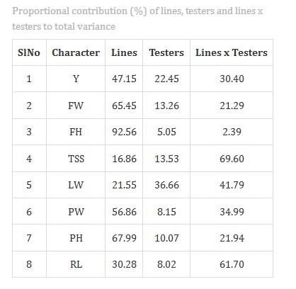
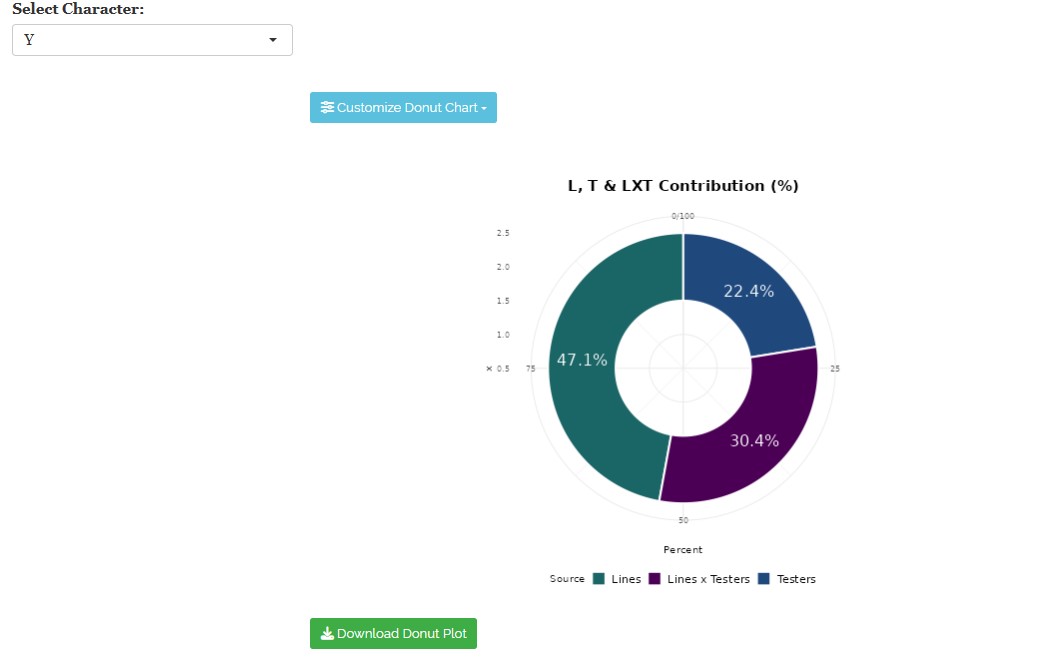
The proportional contribution of Lines, Testers, and the Lines × Testers interaction to total variance shows the relative importance of additive and non-additive effects for each trait. RAISINS presents this as a table (Figure 18) plus three downloadable visualisations: a Donut Chart (Figure 19), a Stacked Bar Chart (Figure 20), and a Radial Bar Chart (Figure 21).
Table 5: Proportional contribution (%) of lines, testers, and lines × testers to total variance
% Contribution: formulae and interpretation
The proportional contribution of each source is computed as:
\[\text{Contribution of Lines (\%)} = \frac{SS_{\text{Lines}}}{SS_{\text{Crosses}}} \times 100\]
\[\text{Contribution of Testers (\%)} = \frac{SS_{\text{Testers}}}{SS_{\text{Crosses}}} \times 100\]
\[\text{Contribution of L} \times \text{T (\%)} = \frac{SS_{L \times T}}{SS_{\text{Crosses}}} \times 100\]
The three add to 100% by construction, since Lines, Testers, and their interaction exhaust the crosses sum of squares. A higher combined contribution of Lines and Testers indicates predominantly additive gene action, while a higher Lines × Testers contribution reflects non-additive gene action.
Interpretation from Figure 18
Lines contributed most to total variance for Fruit Height (92.56%), Plant Height (67.99%), and Fruit Weight (65.45%), indicating predominantly additive gene action for these traits. In contrast, the Lines × Testers interaction contributed most for TSS (69.60%), Rind Length (61.70%), and Locule Width (41.79%), pointing to non-additive effects.
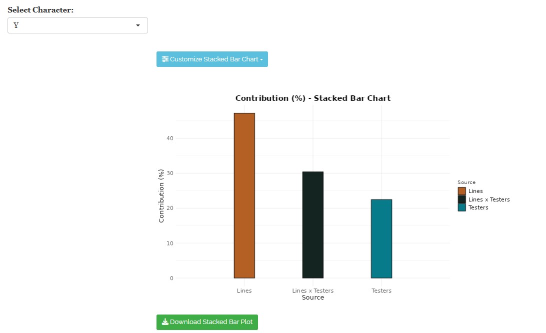
Yield sits between the two: Lines accounted for 47.15%, Lines × Testers for 30.40%, and Testers for 22.45%, indicating a mix of additive and non-additive effects. This is the common case in practice, and it is why the callout in Figure 2 warns that a trait can show both. A breeding programme for yield in this material would need to exploit both good general combiners and specific cross combinations rather than committing entirely to one strategy.
Donut Chart: L, T and L×T contribution (%) for Yield
Stacked Bar Chart: contribution (%) for Yield
Radial Bar Chart: contribution (%) for Yield
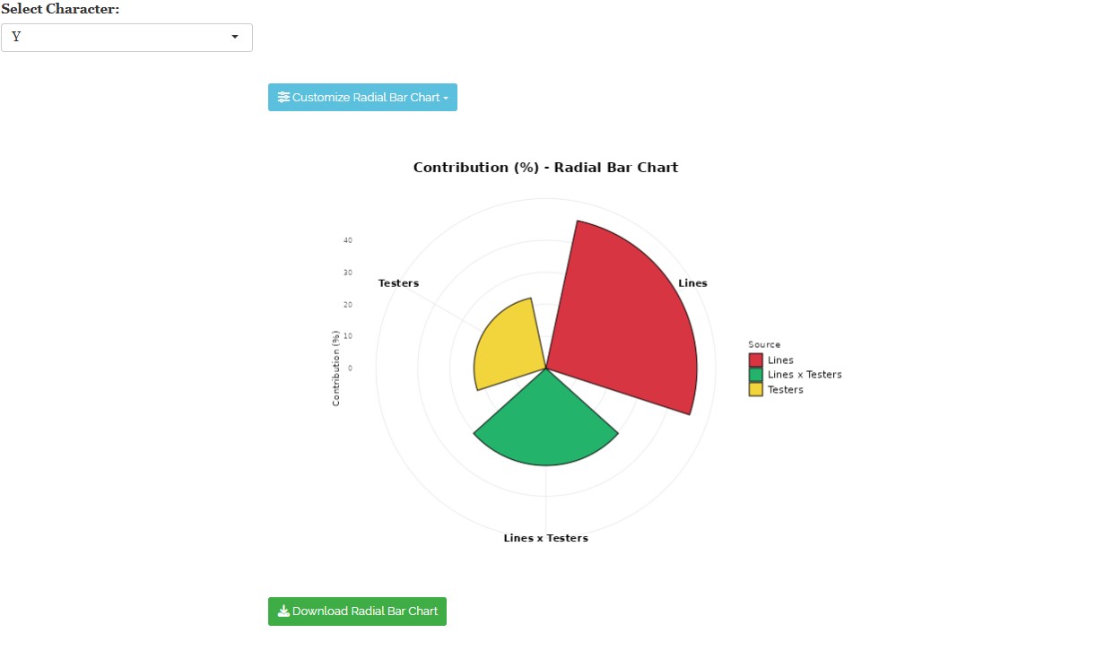
The donut, stacked bar, and radial bar charts for yield visually confirm that Lines (47.1%) contribute the largest share, followed by Lines × Testers (30.4%) and Testers (22.4%). All three charts are customisable and downloadable within RAISINS for reporting.
15 Genetic variance components
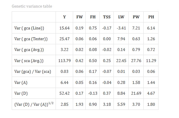
RAISINS estimates genetic variance components including additive variance Var(A), dominance variance Var(D), GCA variances for lines and testers, and SCA variance, along with the Var(D)/Var(A) ratio that determines the nature of gene action for each trait (Figure 22). These are the numbers that settle what the ANOVA only suggested.
Table 6: Genetic variance components
Interpretation from Figure 22
Dominance variance Var(D) exceeded additive variance Var(A) for most traits, including yield (52.42 vs 6.44), Fruit Weight (0.17 vs 0.05), Locule Width (8.84 vs 0.28), Pericarp Width (21.69 vs 1.58), and Plant Height (4.67 vs 1.44), confirming the predominance of non-additive gene action. The Var(D)/Var(A) ratio was highest for Locule Width (5.59) and TSS (3.18), reinforcing dominance effects for these traits.
Var(gca)/Var(sca) ratios were consistently below 1.0 across all traits, indicating that SCA outweighs GCA in governing trait expression. Following the logic of Figure 2, this material is better suited to a hybrid breeding programme than to population improvement, at least for the traits measured here.
16 Genetic divergence parameters and genetic advance
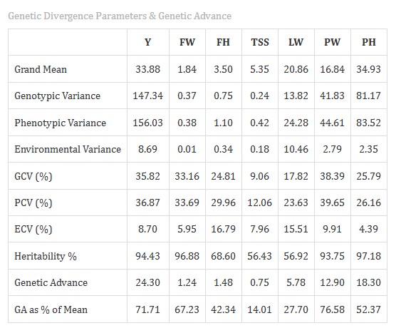
RAISINS estimates key genetic parameters including genotypic and phenotypic variances, heritability, genetic advance, and GCV/PCV for all traits (Figure 23).
Table 7: Genetic divergence parameters and genetic advance
Interpretation from Figure 23
High broad-sense heritability was observed for Plant Height (97.18%), Fruit Weight (96.88%), yield (94.43%), and Pericarp Width (93.75%), indicating these traits are largely under genetic control with minimal environmental influence. Genetic Advance as a percentage of mean was highest for Pericarp Width (76.58%) and yield (71.71%), suggesting selection would be effective for improving them. High heritability coupled with high genetic advance points to additive gene action and a reliable selection response. GCV and PCV values were close for most traits, reflecting low environmental variance and good experimental precision.
A high broad-sense heritability does not by itself justify selection, because it includes both additive and non-additive variance. In this dataset the broad-sense heritability for yield is 94.43% while Var(D) far exceeds Var(A), which means much of that heritability is dominance that will not be transmitted through selfing. Always read heritability alongside the variance components in Section 15 rather than on its own.
17 Heterosis
Heterosis is the superiority of an F₁ hybrid over its parents, and it is the practical payoff the whole analysis has been building towards. Combining ability tells you why a cross performs; heterosis tells you whether it is worth releasing. RAISINS computes three kinds for all p × q crosses, and they form a ladder of increasing severity:
- Mid-parent heterosis asks whether the hybrid beats the average of its two parents. The easiest bar to clear, and mostly of academic interest.
- Heterobeltiosis asks whether it beats the better of its two parents. Harder, and the first bar that matters practically.
- Standard heterosis asks whether it beats the commercial check. The only bar a farmer cares about.
A cross can clear the first two and still fail the third, which is why all three are reported.
17.1 Mid-parent heterosis
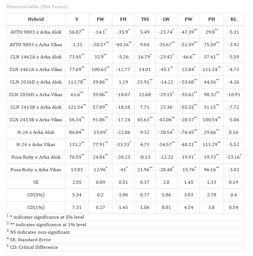
Table 8: Heterosis estimates for all crosses
Heterosis: formulae and interpretation
Mid-parent Heterosis (MPH)
The percentage deviation of the F₁ hybrid mean from the average of its two parents (mid-parent value, MP):
\[MPH (\%) = \frac{\bar{F_1} - MP}{MP} \times 100\]
where \(MP = \frac{P_1 + P_2}{2}\), P₁ = line mean, P₂ = tester mean.
Heterobeltiosis (BPH)
The percentage superiority of the F₁ hybrid over the better parent (BP):
\[BPH (\%) = \frac{\bar{F_1} - BP}{BP} \times 100\]
where BP = max(P₁, P₂) for traits where higher values are desirable, or min(P₁, P₂) for traits where lower values are desirable.
Standard Heterosis (SH)
The percentage superiority of the F₁ hybrid over the standard check cultivar (\(\bar{C}\)):
\[SH (\%) = \frac{\bar{F_1} - \bar{C}}{\bar{C}} \times 100\]
Significance of heterosis estimates is tested using the t-test:
\[t = \frac{\text{Heterosis estimate}}{SE(\text{heterosis})}\]
Significant positive values for yield-related traits indicate true heterosis. Significance is denoted by * (5%) and ** (1%) as superscripts.
Interpretation from Figure 24
Most crosses exhibited positive and significant mid-parent heterosis for yield, confirming genuine hybrid vigour in the material. H-24 × Arka Vikas recorded the highest (131.2**), followed by CLN 2413R × Arka Alok (121.54**) and CLN 2026D × Arka Alok (112.78**). For Fruit Weight, CLN 1462A × Arka Vikas (100.62**) and CLN 2413R × Arka Vikas (91.86**) showed exceptionally high heterosis.
Fruit Height exhibited predominantly negative mid-parent heterosis across all crosses, which may be desirable or not depending on the breeding objective. For Pericarp Width most crosses showed significantly negative heterosis, with H-24 × Arka Alok recording the largest negative value (−76.45**).
17.2 Heterobeltiosis
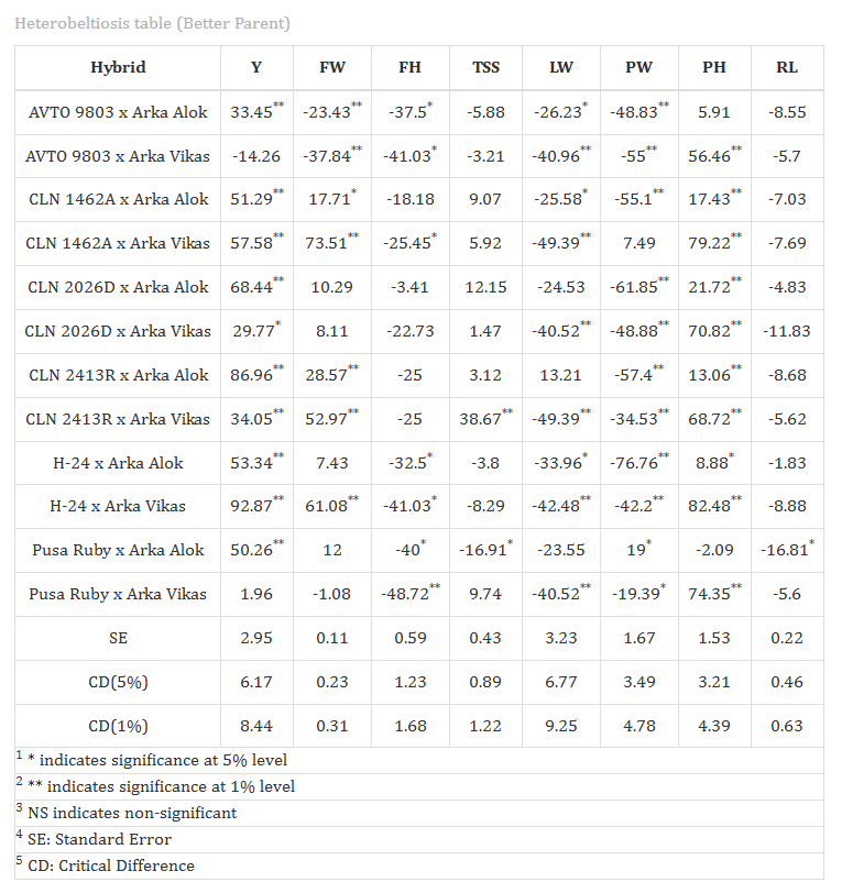
Heterobeltiosis is a more stringent and more practically meaningful measure than mid-parent heterosis, because it compares the hybrid against the better of its two parents rather than their average. A cross with significant positive heterobeltiosis for yield genuinely outperforms both its parents and becomes a priority candidate (Figure 25).
Table 9: Heterobeltiosis estimates
Interpretation from Figure 25
H-24 × Arka Vikas (92.87**), CLN 2413R × Arka Alok (86.96**), and CLN 2026D × Arka Alok (68.44**) exhibited the highest significant positive heterobeltiosis for yield, surpassing their better parent and making them priority candidates for multi-location evaluation. For Fruit Weight, CLN 1462A × Arka Vikas (73.51**) and H-24 × Arka Vikas (61.08**) were outstanding.
Pericarp Width showed predominantly negative heterobeltiosis, with H-24 × Arka Alok (−76.76**) and CLN 2026D × Arka Vikas (−48.88**) the largest negative values. All crosses showed negative heterobeltiosis for Fruit Height. Crosses with non-significant or negative heterobeltiosis for yield are inferior to their better parent and are not recommended for hybrid development.
17.3 Standard heterosis
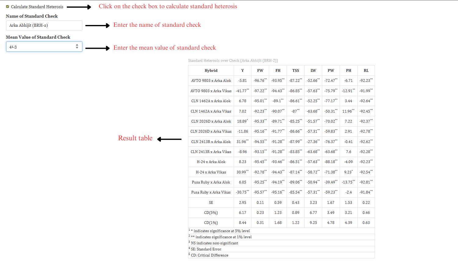
Standard heterosis, also called economic heterosis, measures superiority over a standard commercial check cultivar. It is the most practically relevant form from a breeder’s perspective, because it answers the only question the market asks: does this hybrid beat what farmers can already buy? (Figure 26)
Table 10: Standard heterosis estimates relative to the check
Interpretation from Figure 26
Values greater than zero and statistically significant indicate crosses that outperform the commercial check Arka Abhijit (BRH-2). For yield, CLN 2413R × Arka Alok (31.96**), H-24 × Arka Vikas (30.99**), and CLN 2026D × Arka Alok (18.89*) showed positive standard heterosis, confirming their superiority over the check.
The contrast with the previous tables is worth dwelling on. The majority of crosses showed strongly negative standard heterosis for Fruit Weight, Fruit Height, TSS, Locule Width, and Pericarp Width, meaning the check performs considerably better for these traits despite the impressive mid-parent figures reported earlier. Pusa Ruby × Arka Vikas recorded the most negative standard heterosis for yield (−30.75**), making it the poorest performer relative to the check.
Only crosses with significant positive standard heterosis for yield, here CLN 2413R × Arka Alok and H-24 × Arka Vikas, are advanced to multi-location trials for varietal release decisions. Crosses falling below check performance are not suitable for commercial deployment regardless of how well they beat their own parents.
Read them in order and watch a cross survive or fail each successive test. H-24 × Arka Vikas clears all three: highest mid-parent heterosis, highest heterobeltiosis, and significant standard heterosis. That consistency, together with its top SCA for yield, is what makes it the outstanding candidate in this experiment.
18 Basic plots
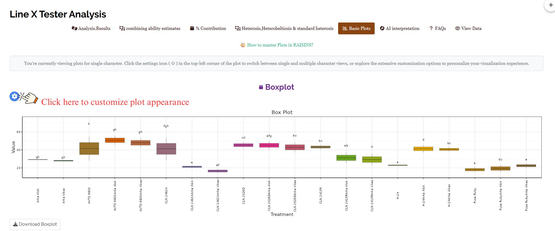
RAISINS provides a suite of publication-ready plots. Once Run Analysis is clicked, all relevant plots appear automatically under the Basic Plots tab. Each plot has a gear icon at the top-left corner for customisation, and can be downloaded in PNG (300 dpi), JPEG, TIFF, PDF, and SVG formats.
18.1 Customising plots
RAISINS provides extensive customisation for all plots. See Figure 27 for an overview of the available options.
Hover over each plot below to see what it shows and when to use it.
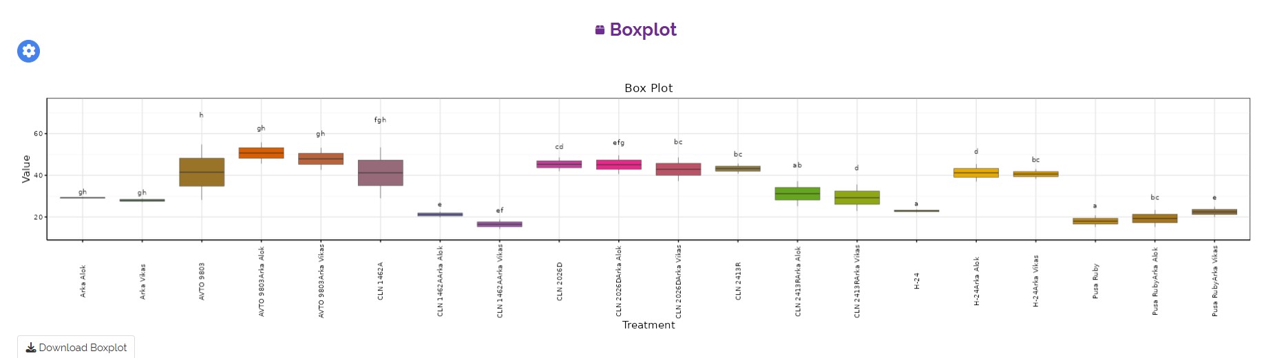
The Boxplot summarises each treatment’s distribution using the median, interquartile range, and whiskers. Colour-coded boxes and compact letter display (CLD) groupings indicate statistical differences. It reveals variability, skewness, and outliers within each treatment group, making it well suited to evaluating the consistency of genotype performance across replicated trials.
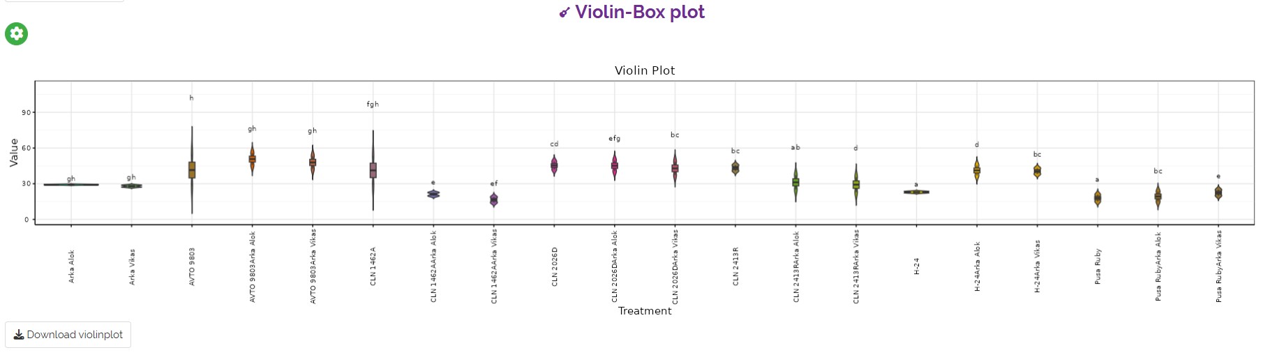
The Violin-Box Plot combines kernel density estimation with embedded boxplot summaries, revealing both distributional shape and key statistics. Colour-coded violins and CLD groupings indicate statistical differences. It displays central tendency, variability, and symmetry at once, useful in breeding trials where the full spread of replicated observations matters for judging genotypic stability.
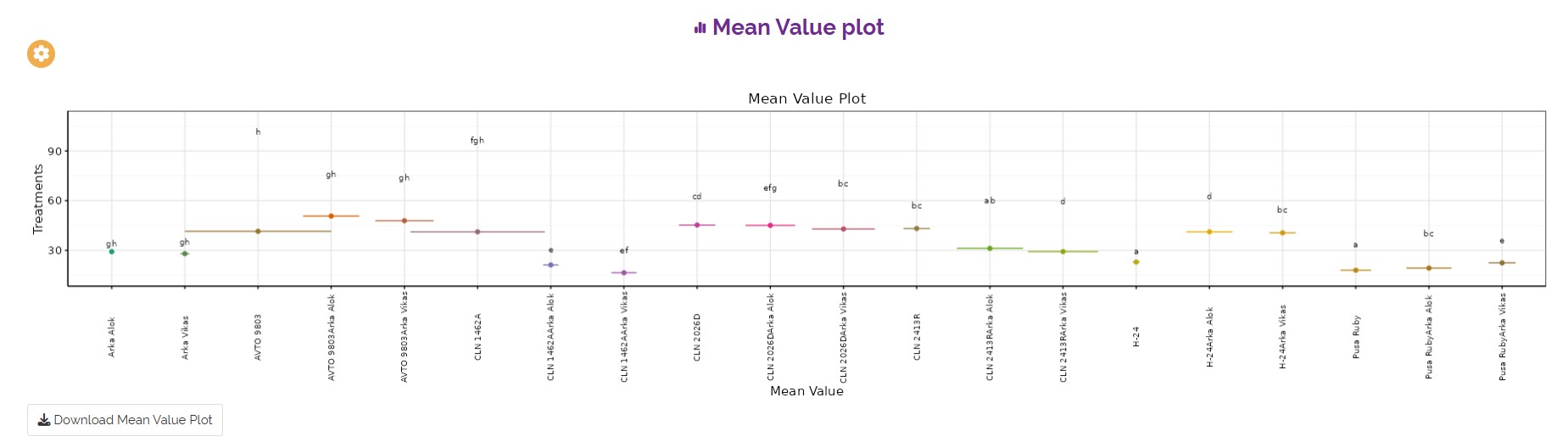
The Mean Value Plot presents treatment means as horizontal points with confidence interval lines, facilitating comparison across many treatments at once. Colour-coding and CLD groupings convey identity and significance. The horizontal layout minimises crowding, showing both mean magnitude and uncertainty, and highlights consistently high or low performers.
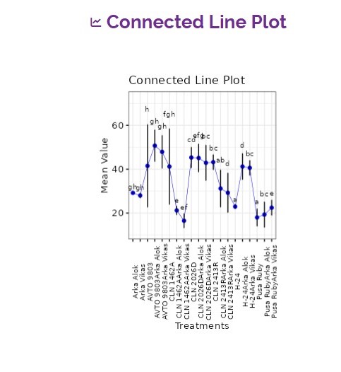
The Connected Line Plot displays treatment means as points linked by a continuous line, with error bars showing standard error and CLD groupings indicating significance. The connecting line helps visualise trends and deviations across successive treatments, combining mean-and-error clarity with trend visualisation.
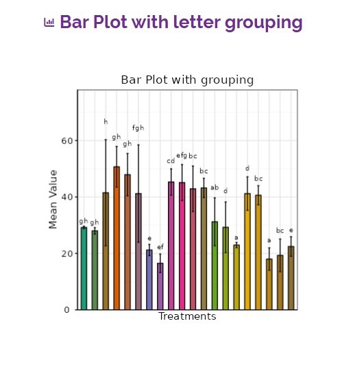
The Bar Plot with Letter Grouping displays treatment means as colour-coded vertical bars with standard error bars. CLD notation above each bar indicates significance, where shared letters denote non-significant differences. It enables rapid comparison of treatment performance and clearly identifies which treatments differ, summarising ANOVA and post-hoc results for breeding trials.
19 Interpretation
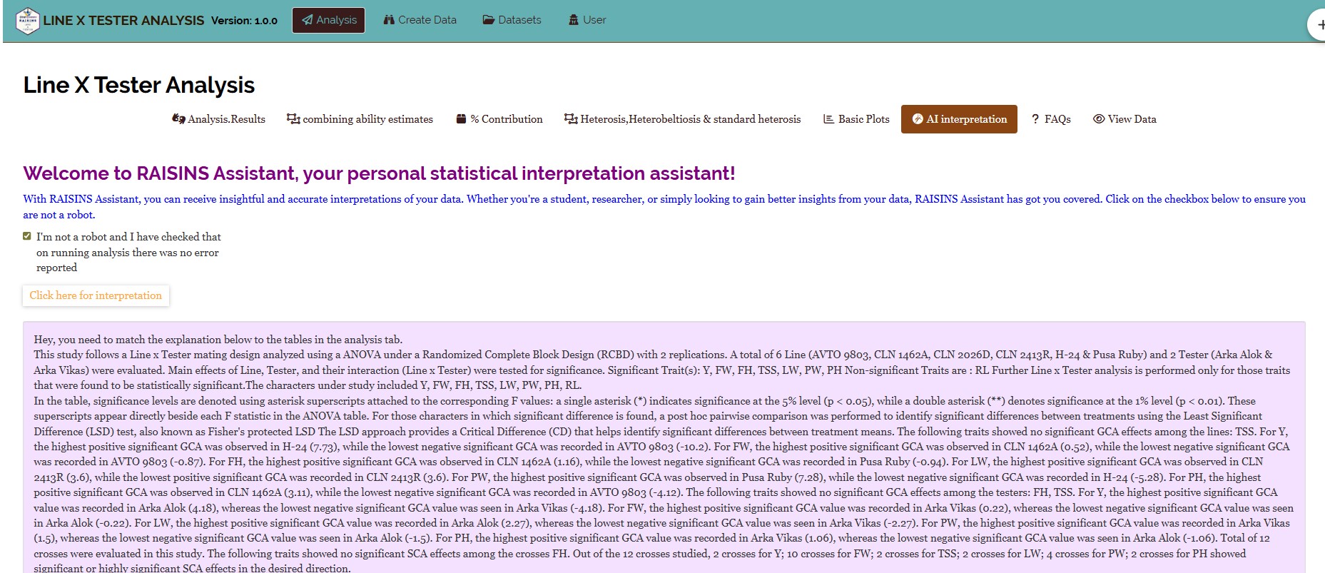
RAISINS provides a clear and concise interpretation of your Line × Tester results to help you understand the findings with ease. The interpretation summarises the combining ability results, identifies statistically significant GCA and SCA effects, indicates the predominant gene action, and presents the findings in a publication-ready format. You can access this from the Interpretation sub-tab of the Analysis tab (Figure 33).
20 Chat with your data using RA-One
RA-One is the built-in conversational assistant for the Line × Tester module, available from the RA-One tab. You ask questions in plain language and it answers using your own analysis rather than generic breeding advice. Every result it discusses is drawn from what the module actually computed. It never invents numbers, and if a value is not available it says so instead of guessing. All answers are in plain English, with no code or software commands.
RA-One works directly with your ANOVA, combining ability, variance component, and heterosis outputs. It can explain what a GCA or SCA effect means for your specific parents and crosses, walk you through why a trait shows additive or non-additive gene action, and interpret the heterosis estimates against your check cultivar. It also handles general concept questions, such as the difference between heterobeltiosis and standard heterosis, or why a good parent need not give a good hybrid, so you can build understanding alongside your results.
The same chat window can also prepare your data. It can build a correctly formatted dataset template (Section 8.2) for you to fill in, or fetch a model dataset (Section 8.3) so you can try the module straight away, so you never need to leave the tab to get a file ready.
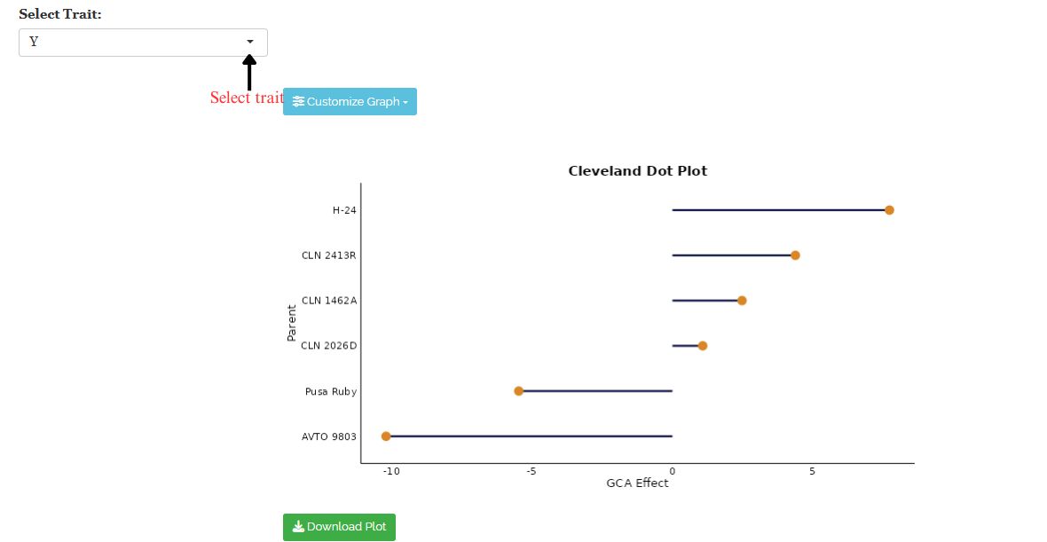
RA-One can also generate plots on request. Ask for a boxplot of the hybrids, a dot plot of GCA effects, or a heatmap of SCA, and the app renders the graphic directly in the chat, where you can view it and refine it by asking for changes.
Within a single conversation, RA-One can interpret your results, build a data template, fetch a model dataset, and produce plots, so most of a routine Line × Tester session can be conducted without ever leaving the chat window.
21 FAQs
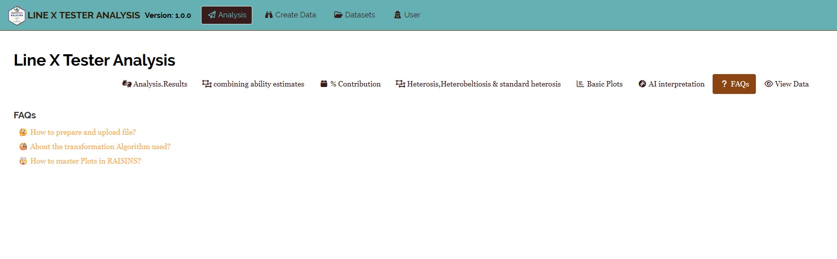
The module includes a dedicated FAQs tab to clarify common doubts and guide you through the features. It offers detailed answers, additional information, and helpful tips for a smooth experience. If you are ever unsure how something works, say how to choose a tester, or why a good general combiner did not give the best hybrid, the FAQs are a good place to start.
22 View data
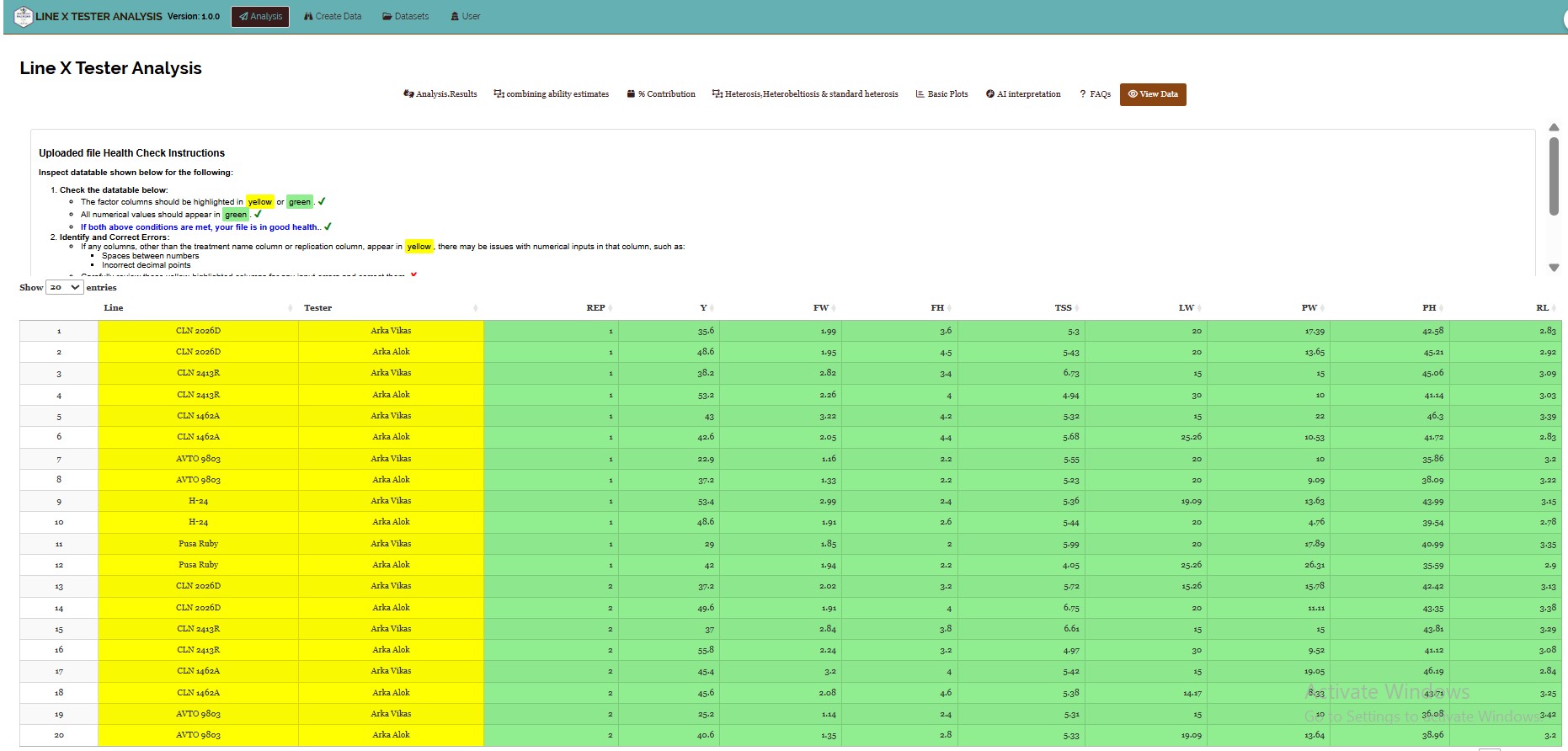
View Data is the primary diagnostic tool for ensuring data integrity before analysis. When you upload your dataset, the system performs an automated Health Check to validate column types, the assignment of Line, Tester, and Replication columns, and overall formatting. For Line × Tester this step matters especially: it confirms that parent rows are correctly recognised through their empty opposite-parent cells, that every line × tester combination is present, and that all trait columns are numeric. Any issues are flagged for correction before you proceed.
23 Wrapping up
Line × Tester analysis rests on one honest question: is this parent good in general, or is this pair good together? Everything else, the ANOVA partition, the variance ratios, the percentage contributions, the three flavours of heterosis, exists only to answer that question fairly and to turn the answer into a breeding decision. RAISINS automates the machinery so you can concentrate on what the answer means for your programme.
In the worked example the verdict was clear: non-additive gene action predominates for most traits, Var(gca)/Var(sca) sits below 1 throughout, and H-24 × Arka Vikas clears every hurdle from SCA through to standard heterosis. That is a hybrid breeding story, not a population improvement one.
If you get stuck at any point, RA-One is available 24 × 7, or write to us at [email protected].
