Repeated Measures One-way ANOVA
A repeated-measures one-way ANOVA tests a single within-subject factor (time/day) measured repeatedly on the same units, removing subject-to-subject variation from the error and checking the sphericity assumption. Read more …
Repeated-measures one-way ANOVA is used when the same experimental units - plants, fruits, animals, soil samples - are measured again and again over time, and the question is whether the response changes from one time point to the next. Because each unit is compared with itself, the unit-to-unit differences are removed from the error, which makes the test far more sensitive than an ordinary one-way ANOVA on the same data. In RAISINS, this analysis can be performed easily without writing any code. This tutorial will guide you step-by-step.
1 What is a repeated-measures one-way ANOVA?
Suppose you pick six fruits and, instead of cutting a fresh fruit for every reading, you measure the same six fruits on day 1, day 2, day 3, day 4 and day 5. On day 1 they average about 43 units; by day 5 they average about 74. The question is simple: does the response really change over time, and between which days?
This is a one-factor question - the only factor is time (Day) - but the data are not ordinary one-factor data. Every fruit appears five times. A fruit that starts high tends to stay high, so the five readings from one fruit are related to each other. An ordinary one-way ANOVA (a CRD) would treat the 30 readings as 30 unrelated fruits, and that is both wrong and wasteful.
A repeated-measures one-way ANOVA handles this properly. It treats each fruit (the subject) as its own baseline and asks whether the within-fruit changes from day to day are larger than the random day-to-day noise.
A repeated-measures one-way ANOVA tests whether a response changes across the levels of one repeated factor (usually time), using each subject as its own control.
2 Subjects and the repeated factor
A one-way repeated-measures design has only two structural columns, and it is worth being clear about both.
The within-subject (repeated) factor is the factor whose levels every subject passes through. In the working example it is Day (day1 to day5). This is the factor being tested.
The subject is the unit that is measured at every level of the repeated factor - here a fruit, identified by sample_ID (1 to 6). The subject is not tested. Its job is to carry the subject-to-subject differences so that they can be removed from the error.
| Column in the example | Role | What it varies | Tested? |
|---|---|---|---|
| Day (day1–day5) | Within-subject (repeated) factor | Across time, within the same fruit | Yes - the Day F-test |
| sample_ID (1–6) | Subject / error stratum | Across fruits | No - removed from the error |
| char1 … char4 | Response variables | The measured characters | One analysis per character |
This is why the repeated-measures analysis is so much more sensitive. In an ordinary one-way ANOVA, the differences between fruits sit inside the error term. In the repeated-measures analysis they are split off into their own stratum, so the Day effect is tested only against the leftover, within-fruit noise. In the working example the between-fruit sum of squares for char1 is about 407, more than twice the within-fruit error sum of squares (about 170). The repeated-measures model takes that 407 out of the error.
The arithmetic looks like a randomised block design with the subject as the block. The difference is randomisation: in an RBD the treatments are randomly assigned within each block, but time points cannot be randomised - day 2 always comes after day 1. That fixed order is what makes readings on nearby days more alike than readings far apart, and it is the reason the extra sphericity check (Section 3) is needed.
3 Sphericity and Mauchly’s test
Repeated-measures ANOVA adds one assumption that ordinary ANOVA does not have: sphericity. It means that the variance of the differences between every pair of time points is about the same - the spread of (day1 − day2) is similar to the spread of (day1 − day5), and so on. Measurements taken close together in time are often more alike than measurements far apart, and when that happens sphericity breaks down.
RAISINS checks this for you with Mauchly’s test of sphericity, reported for every character right under the ANOVA table. For each character it shows Mauchly’s W, its p value, and a verdict:
- ✔ (Assumed) - p is at least α, so there is no evidence against sphericity.
- ✘ (Violated) - p is below α, so sphericity is doubtful.
When sphericity is violated, the uncorrected Day F-test is too liberal - it declares significance too easily. The standard fix is to shrink the degrees of freedom of the F-test, which RAISINS offers through the Sphericity Correction selector:
- Greenhouse–Geisser (GG) - the widely used, cautious correction.
- Huynh–Feldt (HF) - a slightly less conservative alternative. When its correction factor (epsilon) comes out above 1 it is set to 1, and the result is then the same as no correction.
By default RAISINS applies no correction. If any character fails Mauchly’s test, a note under the table says so, and a link in that note takes you straight to the Sphericity Correction selector.
With only two time points there is only one difference, so sphericity holds automatically and Mauchly’s test is not reported. With few subjects and many time points, Mauchly’s test has little power and can miss a real violation. If in doubt, choose Greenhouse–Geisser. It costs little when sphericity holds and protects you when it does not.
4 Assumptions of repeated-measures ANOVA
The analysis is trustworthy only when its assumptions hold. The main ones are listed below.
| Assumption | What it means | How RAISINS helps |
|---|---|---|
| Normality | The model residuals are approximately normally distributed | QQ Plot with Shapiro–Wilk, Anderson–Darling and Kolmogorov–Smirnov tests (Section 14) |
| Sphericity | Variances of the differences between time points are equal | Mauchly’s test and GG / HF corrections (Section 3) |
| Independence of subjects | Different subjects are independent of one another | Ensured by your experimental design |
| Complete, balanced data | Every subject is measured at every time point | Health Check in View Data (Section 20) flags gaps |
Repeated-measures ANOVA expects every subject to be measured at every time point. If a fruit is missing a day, it cannot contribute a complete profile. Check the View Data Health Check (Section 20) before running the analysis.
5 Getting to the module
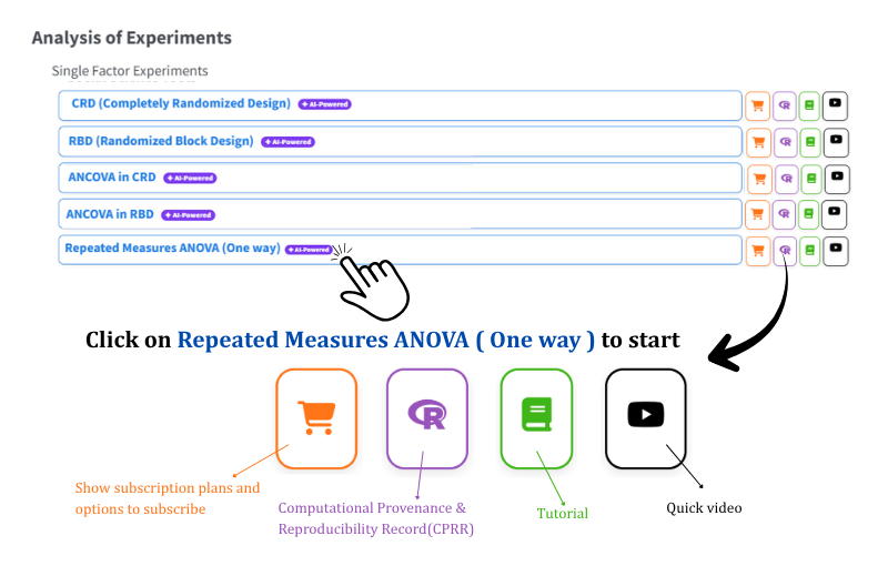
Now that the theory is clear, let us run the analysis. Visit the RAISINS home page at www.raisins.live and go to Analysis of Experiments. In this tutorial we use the Repeated Measures ANOVA (One way) module, shown in Figure 1.
5.1 Computational Provenance & Reproducibility Record
CPRR (Computational Provenance & Reproducibility Record) provides a transparent and comprehensive record. Click on the icon shown in Figure 1 to access CPRR and see the computational workflow behind the analysis. The record for this module states the R version and the exact version of every package used, and names the specific function behind each reported result. CPRR lists every default parameter and decision rule applied by the module and provides runnable R code that reproduces each analytical step, so you can check the results independently in R.
To cite the platform itself in a paper, thesis, or report, use the RAISINS citation, available in APA, Harvard, and BibTeX formats at www.raisins.live/citation.html. That is the primary reference, and for most manuscripts it is all you need.
The CPRR for the repeated-measures one-way ANOVA is at www.raisins.live/module_record/rmanova_oneway.html.
Cite the RAISINS paper as your primary reference for the platform. Add the CPRR as supporting documentation when a journal asks for details of the computing environment, or when you want your methods section to name versions and functions rather than say “analysis was carried out using an online tool.” The CPRR supports the citation and ensures computational reproducibility.
6 Preview mode and Quick Tour
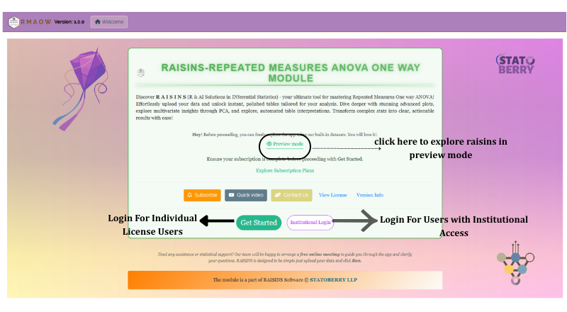
Before subscribing, you can explore the entire module using Preview mode, accessible from the Welcome page. Preview mode loads built-in datasets so you can try every feature (the analysis, Mauchly’s test and the sphericity corrections, multiple comparisons, plots, the multivariate tab, and the RA-One assistant) without uploading your own data. First-time users are also offered a Quick Tour, an interactive, step-by-step walkthrough that highlights each control and explains what it does. You can retake the tour at any time from the Quick Tour tab.
7 A working example
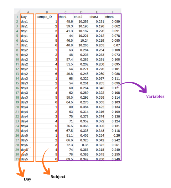
This tutorial uses the Fruit Health Data, the first model dataset bundled with the module (Section 8.3). Six fruits (sample_ID 1 to 6) were each measured on five days (day1 to day5), and four characters (char1, char2, char3, char4) were recorded at every visit - 30 rows in all. Day is the repeated factor and sample_ID is the subject. The question is whether each character changes over the five days, and between which days.
Most of the worked numbers below are for char1, which behaves well on every check. The other three characters are used where they teach something char1 cannot.
8 How to prepare your data
Your analysis is only as good as your data. Feed RAISINS high-quality data and it will deliver powerful insights; feed it messy data and the results will not be trustworthy. You have four routes:
- Create your dataset in MS Excel
- Build your dataset directly within the RAISINS app
- Using the Model datasets in RAISINS as a reference
- Create your dataset using the RA-One chat assistant
8.1 Preparing data in MS Excel
Open a new blank sheet in MS Excel containing only one sheet, and avoid adding any unnecessary content. The dataset should follow a column-based (“long”) format with one row per subject per time point. One column holds the Day/Time label (e.g. day1, day2, …), another identifies the Subject (the unit measured on every day, e.g. 1, 2, 3 …), and every response character occupies its own column. The order of the columns does not matter, because you pick the Day/Time and Subject columns yourself in the Analysis tab. The file can be saved as CSV, XLS, or XLSX, but CSV is recommended as it is lighter and loads faster. For reference, see the structure in Figure 3.
Dataset creation rules
- Column naming convention
- No spaces allowed in column names.
- Use underscores (
_) or full stops (.) for separation. - Avoid symbols and special characters such as %, #.
- Data arrangement
- Start the data towards the upper-left corner.
- Ensure the row above the data is not blank.
- Cell management
- Avoid typing or deleting in cells without data.
- If needed, select the affected cells, right-click, and choose Clear Contents.
- Column relevance
- Name all columns meaningfully.
- Exclude unnecessary columns not required for the analysis.
- Day and subject labels
- Every subject should appear exactly once at every Day/Time point, so each subject has a complete profile.
- Use the same subject label for the same unit on every day - subject 3 on day1 must be subject 3 on day5.
- Keep spelling and capitalisation of all labels consistent throughout.
How to save as CSV in MS Excel
Open your workbook. Ensure your data is arranged properly with only one sheet.
Click the ‘File’ menu. Go to the top-left corner and click File.
Choose ‘Save As’ or ‘Save a Copy’. Select the location where you want to save your file.
Set file type to CSV. In the ‘Save as type’ dropdown, choose CSV (Comma delimited) (*.csv).
Name your file. Enter a relevant file name without spaces (use underscores if needed).
Click ‘Save’. Click Save to export the file.
💡 Tip: Before saving, double-check that your data is on the first sheet and follows the required format: no empty rows above the data, meaningful column names, and a complete Day–Subject layout.
8.2 Prepare using Create Data in RAISINS
If you are unsure about the correct format, do not worry, RAISINS can create the data layout for you. Here is how:
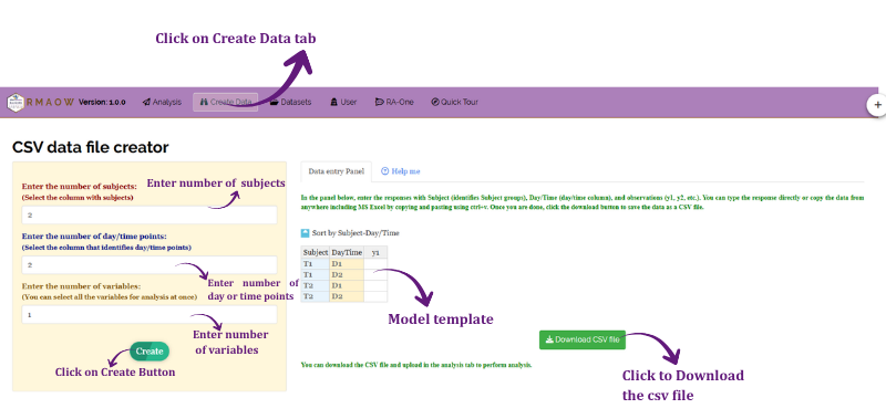
- Navigate to the Create Data tab
- Enter the number of subjects
- Enter the number of day/time points
- Enter the number of variables
- Click the Create button
The model layout appears as shown in Figure 4, with the Day/Time and Subject columns already filled in. You may enter the observations manually into the CSV once downloaded, or paste them straight into the table provided. Once the observations are entered, download the CSV and upload it under Analysis.
8.3 Download Model Datasets
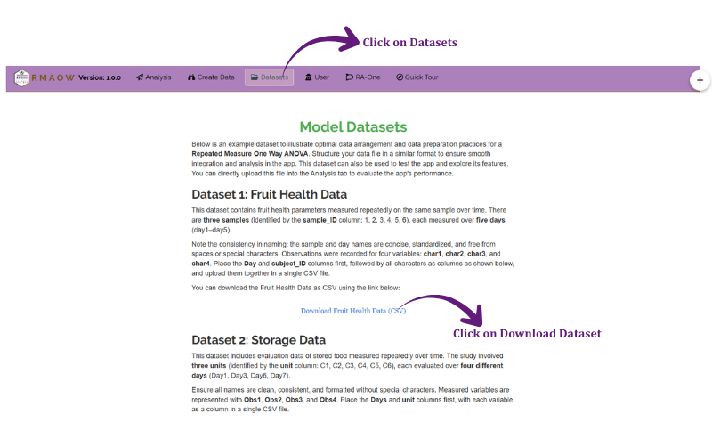
If you are unsure about the required data format or would like to explore the module before using your own data, RAISINS provides three model datasets: Fruit Health Data (6 fruits × 5 days, four characters - the working example), Storage Data (6 units × 4 storage days, four observations), and Soil Data (4 samples × 4 days, six nutrients). To download them:
- Navigate to the Datasets tab
- Click the Download … (CSV) link under the dataset you need
- Save the file to your computer
- Use the model dataset as a reference for preparing your own data or upload it directly to explore the analysis
8.4 Creating a dataset using RA-One chat
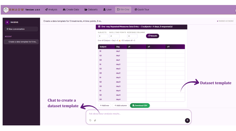
RA-One, the built-in chat assistant, can help you create a properly formatted dataset through a simple conversation. Open the RA-One chat by clicking the chat icon within the app or by heading over to the RA-One tab. Tell it how many subjects, time points and response variables you have, and RA-One will generate a dataset in the required repeated-measures format. You can review it in the chat, download it as a CSV file, and upload it directly under the Analysis tab (Figure 6).
9 The Analysis tab
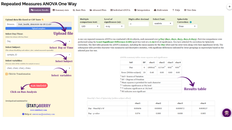
Figure 7 shows the Analysis tab. Upload your prepared file by clicking Browse in the sidebar. Once it is uploaded, three selectors appear:
- Select Day/Time - the column holding the repeated factor (in the example, Day).
- Select Subject - the column identifying each subject, plot or animal measured repeatedly (in the example, sample_ID).
- Select variables - the response characters to analyse, one or many at once (char1 to char4).
A toggle underneath lets you apply a transformation (Section 10) before the analysis. Click Run Analysis!, and a control bar appears above the results with five settings. Change any of them and the results update straight away:
- Multiple comparison test - LSD (default) or TUKEY.
- Level of significance (α) - 0.05 (default) or 0.01.
- Digits after decimal - 1 to 4 (default 2).
- Select Font - the font of the result tables.
- Sphericity Correction - None (default), Greenhouse Geisser, or Huynh Feldt (Section 3). The ⓘ icon beside it opens a short explanation.
The results are spread across the sub-tabs: Analysis Results, Summary stats, Basic Plots, Advanced Plots, Individual ANOVA, Interpretation, Multivariate, FAQs, and View Data.
10 Transformation
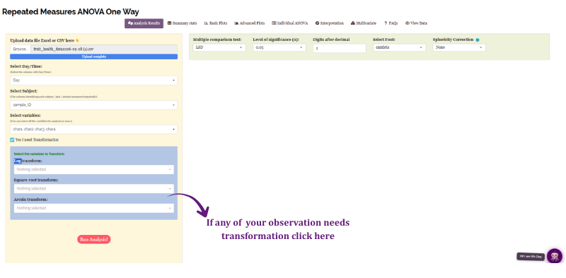
Log, square root, and arcsine transformations are used to make data more normal and to even out uneven variation. Switch on the transformation toggle and pick the variables for each transformation, as shown in Figure 8. The analysis is then run on the transformed values, and the results table shows the original means with the transformed means in parentheses.
Logarithmic transformation (base 10) makes a right-skewed distribution more symmetrical. It suits positive, continuous data whose variance grows with the mean. If a column contains zero or negative values, RAISINS first shifts it so that its smallest value becomes 1.
Square root transformation stabilises variance for non-negative count data, where the variance increases with the mean. If a column contains zeros, 0.5 is added before taking the root. Negative values are rejected with a warning.
Arcsine transformation (the angular transformation) is for proportions between 0 and 1. It takes the inverse sine of the square root of each proportion. Values of exactly 0 or 1 are nudged inwards by 1/(4n) first, and values outside 0–1 are rejected with a warning.
After choosing the appropriate transformation, proceed to Section 11 for the analysis.
11 Analysis results
Once you click Run Analysis!, the repeated-measures one-way ANOVA is fitted for every selected character. The model RAISINS fits is
\[\text{response} \sim \text{Day} + \text{Error}(\text{Subject}/\text{Day})\]
which reads: the response depends on Day, and the repeated measurements are nested inside each Subject. The Analysis Results sub-tab shows three tables in order - the ANOVA summary, Mauchly’s test of sphericity, and the detailed results for Day.
11.1 Table 1: ANOVA summary
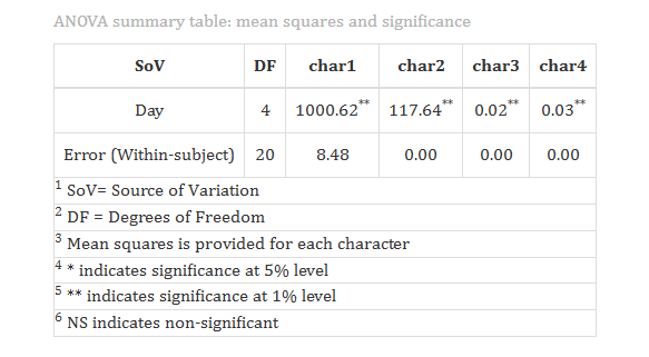
The ANOVA summary has one column per character and two rows: Day and Error (Within-subject). For each it gives the degrees of freedom (DF) and the mean square, and the Day mean square carries a significance mark: ** at the 1% level, * at the 5% level, and NS for non-significant. With 6 subjects and 5 days, Day has 5 − 1 = 4 DF and the within-subject error has (5 − 1) × (6 − 1) = 20 DF.
For char1, the Day mean square is 1000.62** against a within-subject error mean square of 8.48. Their ratio is the F statistic, 117.95, so the change over time is highly significant. All four characters are significant (**).
The between-subject row (the fruit-to-fruit variation) is deliberately not shown. In a one-way repeated-measures design it is not a test term - it is only the variation that has been removed from the error (Section 2).
char2, char3 and char4 are measured in small units, so with the default 2 decimals their error mean squares print as 0.00. That is a rounding effect, not a zero error. Set Digits after decimal to 4 and the values appear (for example, char3’s error mean square is 0.0007).
If you choose Greenhouse Geisser or Huynh Feldt, the DF shrink - for char1 under GG, from 4 and 20 to about 2.61 and 13.07 - and the mean squares are recalculated on those corrected DF. The F statistic itself does not change; only its reference distribution, and so its p-value, does.
11.2 Table 2: Mauchly’s test of sphericity
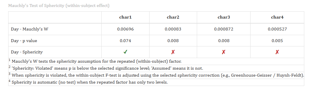
This table has three rows for the Day effect - Mauchly’s W, its p value, and the Sphericity verdict - and one column per character. In the working example:
| char1 | char2 | char3 | char4 | |
|---|---|---|---|---|
| Mauchly’s W | 0.00696 | 0.00083 | 0.000872 | 0.000527 |
| p value | 0.074 | 0.008 | 0.008 | 0.005 |
| Sphericity | ✔ | ✘ | ✘ | ✘ |
char1 passes (p = 0.074 is above 0.05), so its uncorrected test can be used as it is. char2, char3 and char4 fail, so a note appears under the table: Sphericity correction needed. Choose Greenhouse Geisser in the Sphericity Correction selector (the link in the note takes you there) and the Day tests are recomputed with corrected DF.
Here the conclusions survive the correction. Under Greenhouse–Geisser, char1 is still p < 0.001 (epsilon = 0.65), and char3 - the weakest effect - is still p = 0.0015 (epsilon = 0.29). But you only know that after applying the correction, which is why the check matters.
The Sphericity Correction selector applies to every character in the run. If some characters pass Mauchly’s test and some fail, the cautious choice is to apply Greenhouse–Geisser to all of them. It barely changes a character that already satisfies sphericity. For char1, whose Huynh–Feldt epsilon exceeds 1, HF gives exactly the uncorrected result.
11.3 Table 3: Detailed results for Day
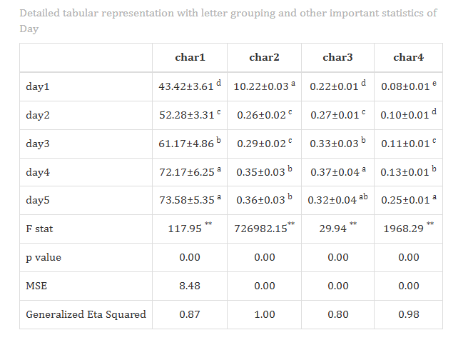
This is the table most people report. For every day and character it gives the mean ± SD and a letter grouping, followed by four summary rows: the F stat, the p value, the MSE (the within-subject error mean square) and the Generalized Eta Squared effect size. Two toggles above the table switch the ± SD and the letter grouping on and off. For char1, with the default LSD test at α = 0.05:
| Day | char1 (mean ± SD) | Group |
|---|---|---|
| day1 | 43.42 ± 3.61 | d |
| day2 | 52.28 ± 3.31 | c |
| day3 | 61.17 ± 4.86 | b |
| day4 | 72.17 ± 6.25 | a |
| day5 | 73.58 ± 5.35 | a |
| F stat | 117.95** | |
| MSE | 8.48 | |
| Generalized Eta Squared | 0.87 |
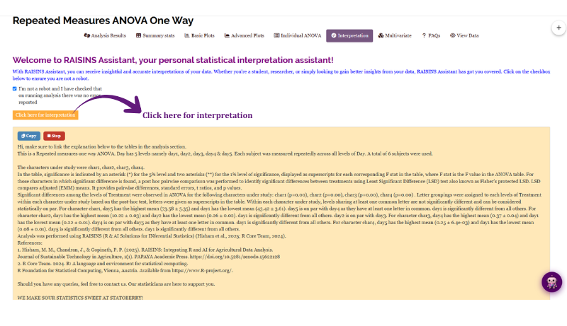
Days that share a letter are not significantly different; days with no letter in common are. The letter a always goes to the highest mean. So char1 rises significantly from day1 to day2 to day3 to day4, and then levels off: day4 and day5 share a and do not differ. The generalized eta-squared of 0.87 says that time accounts for most of the variation in char1. Letters are shown only when the Day effect is significant at your chosen α - if it is not, the grouping column is left blank.
Interpretation of Figure 11
char1 changed significantly over the five days (F(4, 20) = 117.95, p < 0.001, generalized η² = 0.87), and Mauchly’s test gave no evidence against sphericity (W = 0.007, p = 0.074). Mean char1 increased from 43.42 on day1 to 72.17 on day4, with each of the first four days significantly different from the next (LSD, α = 0.05). There was no further significant change between day4 (72.17) and day5 (73.58).
A tiny difference can be statistically significant, and a large, valuable difference can miss significance in a small trial. Always read the size of the difference in the means alongside the significance mark, and ask whether it matters in practice - here, whether the 1.4-unit gain from day4 to day5 is worth waiting a day for.
Downloading the results. Below the tables you can download the Analysis Results as a report in HTML, PDF or Word format. The report carries the ANOVA summary, the Mauchly’s test table with the correction you chose, and the detailed Day table.
A quick glossary of the result columns
Overview of the ANOVA and detailed tables
- Sources of variation
Day: the within-subject (repeated) factor - differences between time points.
Error (Within-subject): the day-to-day noise left inside each subject after the Day effect; the denominator of the Day F-test.
- Test statistics
DF (Degrees of Freedom): (days − 1) for Day and (days − 1) × (subjects − 1) for the error. Both are reduced when a Greenhouse–Geisser or Huynh–Feldt correction is applied.
Mean square: a sum of squares divided by its DF. The F statistic is the Day mean square divided by the error mean square.
Mauchly’s W: the sphericity test statistic; values near 1 are consistent with sphericity.
Generalized eta-squared: the effect size reported by the model - the share of variance attributable to Day.
- Descriptive columns
Mean ± SD: the day mean and its standard deviation across subjects. With a transformation, the transformed mean is shown in parentheses.
Letter grouping: days sharing a letter are not significantly different; derived from the LSD or TUKEY comparison at the chosen α.
MSE: the within-subject error mean square.
12 Summary statistics
The Summary stats sub-tab gives you the full descriptive picture before you lean on the inference. For every Day and each character it reports the number of subjects (N), Mean, Standard Deviation (SD), Standard Error (SE), Minimum, Maximum, Coefficient of Variation (CV %), Skewness and Kurtosis, with Copy / Excel / CSV / PDF buttons to export each table (Figure 12).
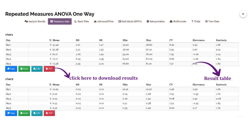
For char1, the day means climb from 43.42 (SE 1.47) to 73.58 (SE 2.19), and the CVs stay between about 6 % and 9 %, so the six fruits are measured consistently. Skewness is close to 0 on every day.
Now look at char2. On day1 its mean is 10.22, and from day2 to day5 it is between 0.26 and 0.36 - about 40 times smaller. A real change of that size in one day is implausible. The day1 values (10.187 to 10.255) look like a data-entry slip, most likely a stray leading “10”. This one issue explains why char2 has an absurd F statistic (over 700,000). It also explains why char2 dominates the multivariate analysis (Section 16). If this were your data, you would check the field notes and correct the file before trusting any char2 result.
The ANOVA answers “are the differences bigger than the noise?” - the Summary stats show you what the means and the noise actually are. Reading them first quickly reveals data-entry problems, like char2’s day1, that would otherwise distort everything downstream.
13 Basic plots
The Basic Plots sub-tab turns your results into quick, publication-ready charts. Five plot types are available as clickable icons - Boxplot, Violin Plot, Mean Value Plot, Connected Line Plot and Bar Plot - and each one is drawn the moment you click it (Figure 13). A settings panel lets you customise the display mode (one character or all characters at once), titles and labels, colours, what is shown or hidden, themes, axes, grid and legend. When you are happy, choose a format (PNG, JPEG, TIFF, PDF or SVG), set the size and DPI, and download.
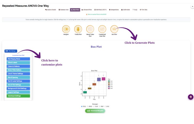
The letters above each day are the same letter groupings as in Table 3 (Section 11.3) - days that share a letter are not significantly different. The Connected Line Plot is especially useful here, because it joins the day means in time order and shows the shape of the change - for char1, a steady rise that flattens between day4 and day5.
14 Advanced plots
The Advanced Plots sub-tab offers seven more graphics: Summary Plot, Advanced Raincloud Plot, Raincloud Plot, Circular Plot, QQ Plot, Distribution Plot and Pair Plot. Pick the response variable, click a plot icon, refine it through its settings panel, and download (Figure 14).
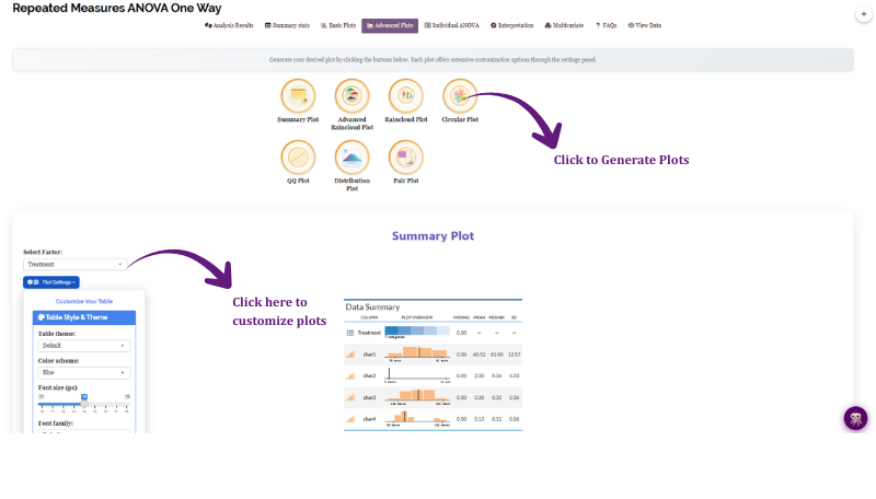
The QQ Plot is the module’s normality check. It plots the model residuals - what is left after removing the day effect and each subject’s own level - against the values a normal distribution would give. If the points follow the straight line, the normality assumption holds. Tick Show Normality Tests to print the Shapiro–Wilk test on the plot (the default), and optionally Anderson–Darling and Kolmogorov–Smirnov.
In the working example the residuals of char1 pass comfortably (Shapiro–Wilk p = 0.66) and char2 also passes (p = 0.19), but char3 (p = 0.016) and char4 (p = 0.003) show some departure from normality. For char3 and char4, look at the QQ plot to see which points stray from the line. Consider a transformation (Section 10) if the departure is clear, and be more cautious with borderline p-values.
With only 30 residuals, a single unusual reading can push the Shapiro–Wilk p-value below 0.05. Always read the test together with the QQ plot - a p-value just under 0.05 with points hugging the line is less worrying than a clear curve.
15 Individual ANOVA
The Individual ANOVA sub-tab shows the complete classical ANOVA table for one selected character at a time, plus every pairwise comparison between days (Figure 15). The ANOVA table lists Day and Error (Within-subject) with their DF, Sum of Squares (SS), Mean Sum of Squares (MSS), F value and p value. This sub-tab has its own report download.
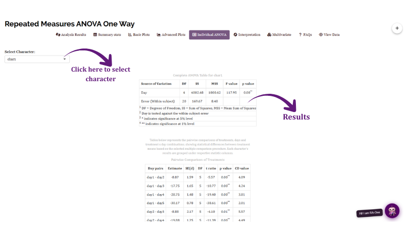
For char1: Day has SS 4002.48 on 4 DF (MSS 1000.62), and the within-subject error has SS 169.67 on 20 DF (MSS 8.48), giving F = 117.95, p < 0.01.
The pairwise comparison table lists every pair of days with its Estimate (the difference in means), SE(d), DF, t ratio, p value and critical difference. With LSD the last column is the CD value, and with TUKEY it is the HSD value. A pair is significantly different when the absolute estimate exceeds its CD. For char1 with LSD:
| Day pairs | Estimate | SE(d) | DF | t ratio | p value | CD value |
|---|---|---|---|---|---|---|
| day1 - day2 | −8.87 | 1.59 | 5 | −5.57 | 0.00** | 4.09 |
| day2 - day3 | −8.88 | 2.17 | 5 | −4.10 | 0.01** | 5.57 |
| day3 - day4 | −11.00 | 2.14 | 5 | −5.13 | 0.00** | 5.51 |
| day4 - day5 | −1.42 | 0.91 | 5 | −1.56 | 0.18NS | 2.33 |
(Only the consecutive days are shown here; the app lists all ten pairs.) The last row is the important one: day4 and day5 differ by only 1.42, which is less than the CD of 2.33, so they are not significantly different - exactly why they share the letter a in Table 3. Switch to TUKEY and the thresholds widen (the HSD for day4 − day5 is 3.64), because Tukey protects against false positives across all ten comparisons at once. Here Tukey gives the same letter grouping as LSD.
In a repeated-measures design, each pairwise comparison uses the actual day-to-day differences of the same subjects. So every pair gets its own standard error, based on how consistently the subjects changed between those two days, with DF = subjects − 1 = 5. This is why the CD is not a single number, as it would be in a CRD or RBD. The pairs with the most consistent changes (day1 − day5, SE(d) 0.78) have the smallest CD, and the most erratic pairs (day2 − day3, SE(d) 2.17) have the largest. Because these comparisons do not rely on the sphericity assumption, the choice of sphericity correction does not change them.
16 Multivariate analysis
When you record several characters, you may want to rank the days using all of them together rather than one at a time. The Multivariate sub-tab does this with Principal Component Analysis (PCA) on the day means of the characters you select (at least three). It reports the eigenvalues (how much variance each principal component explains), the variable loadings (how each character contributes), and a PCA-based index score for each day on PC1 and PC2, rescaled to 0–1 so the days are easy to compare (Figure 16).
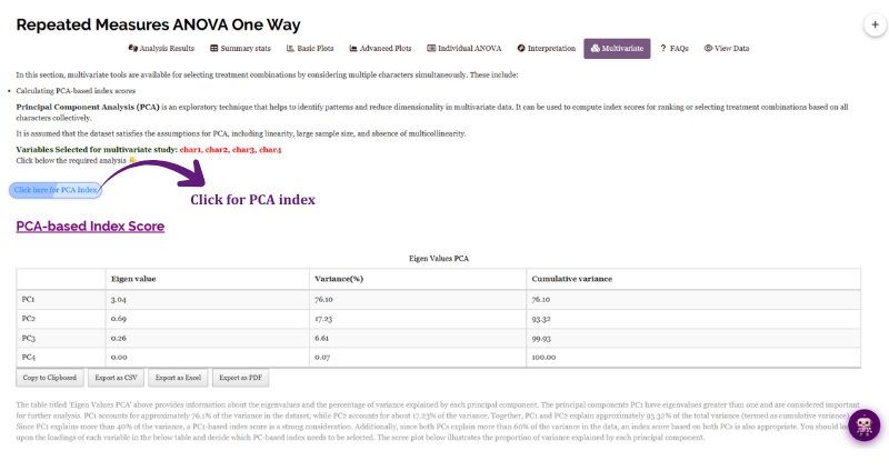
With all four characters, PC1 explains 76.10 % of the variance and PC2 17.23 % (cumulative 93.32 %), so the app suggests that an index based on PC1 is well supported. char1, char3 and char4 load on PC1 with one sign and char2 with the other, so PC1 separates day1 - where char2 is suspiciously high (Section 12) - from the later days.
This is a good example of why the multivariate tab must be read with care. A single data-entry problem in one character can dominate the whole index. Correct the data first, then rerun the PCA.
The PCA index is a convenient way to combine several characters into one score, but it is an exploratory ranking tool, not a hypothesis test. The ANOVA tables remain the basis for inference.
17 Interpretation
RAISINS provides a clear and concise interpretation of your results. In the Interpretation sub-tab, tick the characters you want and click the button to generate a write-up. It summarises whether the Day effect is significant for each character, explains the letter groupings, mentions the multiple-comparison test and the sphericity correction you used, and presents the findings in a publication-ready form. Copy and Stop buttons let you copy the text or stop it early (Figure 17).
18 Chat with your data using RA-One
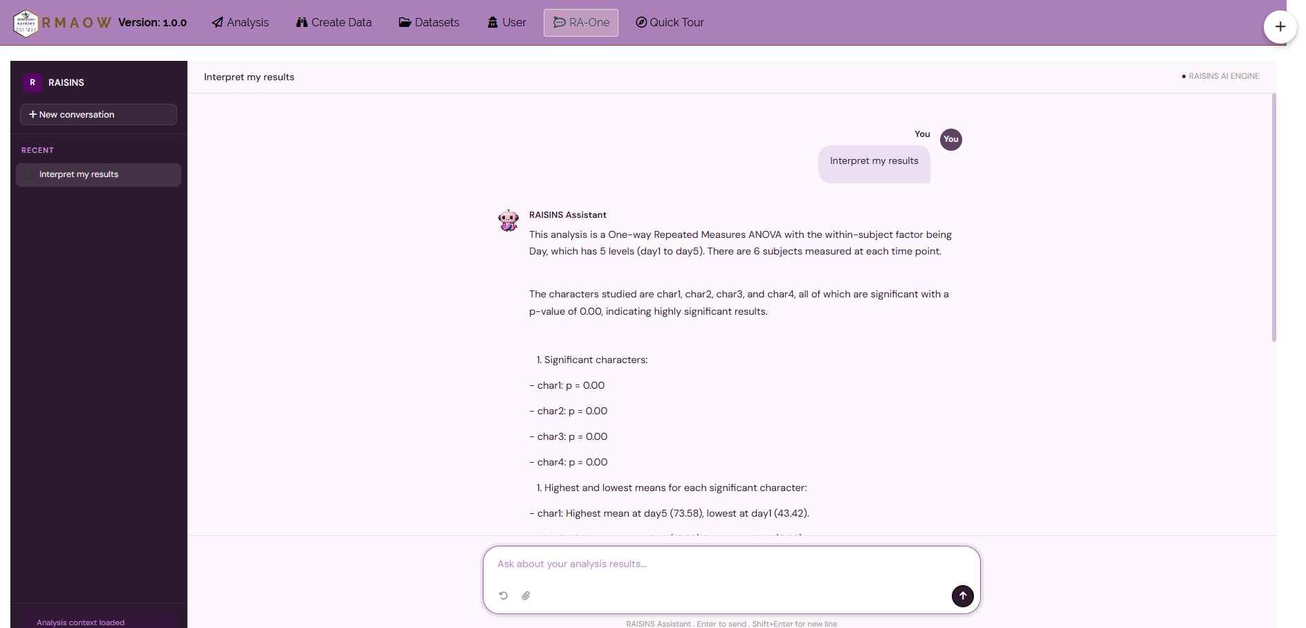
RA-One is the built-in conversational assistant for this module, available from the RA-One tab and the chat icon. You ask questions in plain language and it answers using your own analysis rather than generic statistical advice. Every result it discusses is drawn from what the module actually computed - it does not invent numbers, and if a value isn’t available it says so. Answers are in plain English, with no code.
It can explain what the Day effect means for your data, why a sphericity correction was or wasn’t needed, how to read the letter groupings, and answer general questions - subjects versus repeated factors, effect sizes, or when to choose Tukey over LSD (Figure 18).
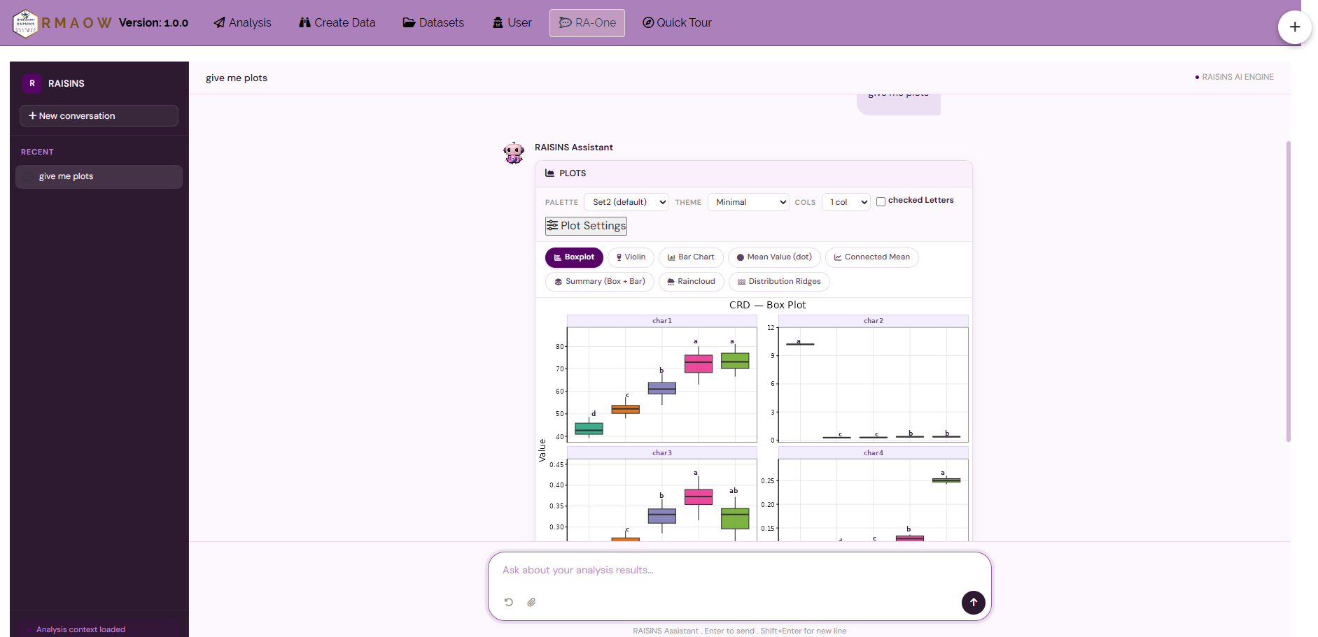
The same chat can also prepare your data - build a dataset template (Section 8.4) or fetch a model dataset (Section 8.3) - and generate plots on request: boxplots, violin plots, bar plots, mean-value and connected line plots, raincloud, distribution and summary plots. The plot appears directly in the chat, and you can refine it by asking for changes (Figure 19).
Within a single conversation, RA-One can interpret your results, build a data template, fetch a model dataset, and produce plots - so most of a routine analysis session can be conducted without leaving the chat window.
19 FAQs
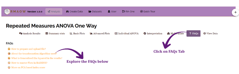
The module includes a dedicated FAQs section to clarify common doubts - when a sphericity correction is needed, how to read Mauchly’s test, how to choose between LSD and TUKEY, and how to lay out your data. If you are ever unsure how something works, the FAQs are a good place to start.
20 View data
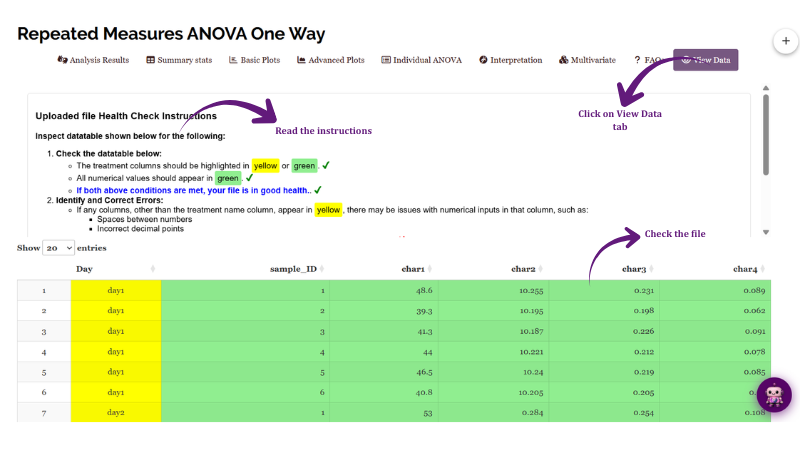
View Data is the primary diagnostic tool for ensuring data integrity before analysis. When you upload a dataset, the system runs an automated Health Check that validates column types and formatting. For a repeated-measures design this matters more than usual. It confirms that the Day/Time and Subject columns are read as labels, that every subject has a value at every time point, and that all response columns are numeric with no missing or badly formatted entries.
21 Wrapping up
The repeated-measures one-way ANOVA answers one question: does the response change over time? The rest - the Error(Subject/Day) stratum, Mauchly’s test, the sphericity corrections, the pairwise comparisons - makes sure that question is answered fairly when the same units are measured again and again. In the working example, char1 rose steadily for four days and then levelled off. The Summary stats also caught a likely data-entry slip in char2 before it could mislead the conclusions.
If your design is different, the companion modules are there: the two-way repeated-measures ANOVA when you also compare treatments over time, and the one-way ANOVA (CRD/RBD) when each unit is measured only once. And if you get stuck at any point, RA-One is available 24 × 7, or write to us at [email protected].
