Split Plot (2,1) Analysis
Two factors in the main plots, one in the sub plots, and two error terms. This tutorial shows how to run a Split Plot (2,1) analysis in RAISINS, from data preparation to the reporting of results… Read more …
A Split-Plot (2,1) design is used when an experiment involves three factors, with two factors requiring larger experimental units and a third factor that can be applied to smaller experimental units. Since the factors are assigned and randomised at two different plot sizes, the design involves two distinct error terms. Appropriate statistical inference therefore requires each source of variation to be tested against its corresponding error term. This tutorial introduces the structure and principles of the Split-Plot (2,1) design and provides a step-by-step demonstration of its analysis using RAISINS, covering data preparation, analysis, results interpretation, graphical visualisation, and reporting of findings.
1 What is a Split Plot (2,1) design?
Certain experimental factors cannot be feasibly applied to small experimental units. Consider a field experiment evaluating three irrigation methods, two ploughing methods, and three fertilizer doses on a wheat crop.
Irrigation imposes a constraint on the experimental layout because adjacent small plots cannot be irrigated at different rates without the risk of lateral movement of water through the soil profile, which may confound the treatment effects. Therefore, each irrigation method is assigned to a large main plot served by its own supply channel.
Ploughing is subject to a similar constraint, as mechanised tillage is impractical on small experimental units and may affect neighbouring plots. Hence, ploughing methods are also assigned to main plots.
In contrast, fertilizer doses do not impose such restrictions and can be applied independently to smaller experimental units without affecting adjacent plots. Fertilizer is therefore assigned to the subplots.
This arrangement forms a Split-Plot (2,1) design, in which irrigation and ploughing constitute the two main-plot factors, while fertilizer constitutes the subplot factor.
Where such practical constraints exist, the experiment is laid out in two stages. First, each block is divided into large main plots, and the combinations of the two main-plot factors are randomly allocated to these plots. Each main plot is then subdivided into smaller subplots, and the levels of the unconstrained factor are randomly allocated to the resulting subplots.
This arrangement constitutes a split-plot design. When two factors are assigned to the main plots and one factor is assigned to the subplots, the design is referred to as a Split-Plot (2,1) design.
The factors are randomised at two distinct plot sizes, resulting in two stages of randomisation and two separate experimental error terms. Each treatment effect must therefore be evaluated against its appropriate error term.
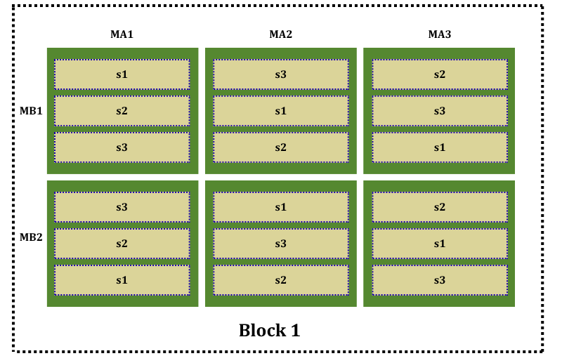
MA1, MA2, MA3) is crossed with main-plot factor B at two levels (MB1, MB2), giving six main plots within the block, shown in green. Each main plot is then divided into three sub plots (s1, s2, s3) to receive the three levels of the sub-plot factor C, giving eighteen sub plots in all. The labels are set out in order for legibility; in the experiment itself the six main-plot combinations are allocated at random within the block, and the sub-plot levels are randomised afresh within every main plot.
1.1 Key principles
Main-plot factors: Factors A and B require large experimental units and are assigned to the main plots.
Subplot factor: Factor C can be applied to smaller experimental units and is assigned to the subplots.
Two error terms: Main-plot and subplot effects are evaluated using their respective error terms.
Precision: Main-plot effects generally have lower precision than subplot effects.
2 The statistical model
Let the number of levels of main-plot factor A be \(a\), the number of levels of main-plot factor B be \(b\), and the number of levels of subplot factor C be \(c\). Suppose the experiment is conducted in \(r\) blocks. Each block contains \(a \times b\) main plots, and each main plot is further divided into \(c\) subplots. Therefore, the total number of observations is
\[N = rabc.\]
For example, the dataset used later in this tutorial has \(a = 2\), \(b = 2\), \(c = 2\), and \(r = 4\), giving
\[N = 4 \times 2 \times 2 \times 2 = 32\]
observations.
Because factors A and B are assigned to the main plots, whereas factor C is assigned to the subplots, the analysis has two distinct strata corresponding to the two stages of randomisation. The model can be represented schematically as
\[\begin{aligned} y =\;& \mu + R + A + B + (A \times B) + E_a \\ &+ C + (A \times C) + (B \times C) + (A \times B \times C) + E_b, \end{aligned}\]
where \(\mu\) is the general mean, \(R\) represents the block effect, \(A\) and \(B\) are the main-plot factors, \(C\) is the subplot factor, and \(E_a\) and \(E_b\) denote the main-plot and subplot error terms, respectively.
2.1 Main-plot stratum
The main-plot stratum contains the variation associated with the assignment of factors A and B to the main plots. It includes the effects of A, B, and their interaction A \(\times\) B, which are evaluated using the main-plot error (\(E_a\)).
2.2 Subplot stratum
The subplot stratum contains the variation generated by the second stage of randomisation, in which factor C is assigned to the subplots within each main plot. It includes the effects of C, A \(\times\) C, B \(\times\) C, and A \(\times\) B \(\times\) C, which are evaluated using the subplot error (\(E_b\)).
The two error terms are therefore not interchangeable. The main-plot error represents variation among main plots within blocks, whereas the subplot error represents the additional variation among subplots within the main plots. This distinction is a direct consequence of the two stages of randomisation and is essential for obtaining valid tests of significance.
In a Split-Plot (2,1) design, main-plot effects are tested against the main-plot error, whereas subplot effects and interactions involving the subplot factor are tested against the subplot error. Using a single pooled error term for all effects would ignore the randomisation structure of the experiment and can lead to incorrect statistical inference.
The validity of a Split-Plot (2,1) analysis depends primarily on the correct implementation of its experimental structure. Factors A and B should be randomly assigned to the main plots, while factor C should be independently randomised to the subplots within each main plot. This two-stage randomisation is what defines the split-plot structure and determines the appropriate error terms for testing the treatment effects.
The analysis also assumes that the errors are approximately normally distributed with reasonably constant variance within the respective main-plot and subplot strata. Block effects are assumed to act additively, without altering the treatment effects. For a balanced analysis, all combinations of A, B, and C should be represented in every block without missing observations.
These assumptions can be assessed using appropriate residual plots and diagnostic methods (Section 12). If substantial departures from the assumptions are observed, an appropriate data transformation may be considered (Section 9).
3 Partition of the variation and the two error terms
The analysis of variance follows the two stages of randomisation in the Split-Plot (2,1) design. Variation is therefore partitioned into a main-plot stratum and a subplot stratum, each with its own error term.
The main-plot stratum accounts for the variation among the main plots within blocks. It contains the effects of the two main-plot factors, A and B, and their interaction A × B. The remaining variation among main plots is represented by Error(a). Therefore, the effects of A, B, and A × B are tested against Error(a).
The subplot stratum accounts for the additional variation among subplots within the main plots. It contains the effect of the subplot factor C and the interactions A × C, B × C, and A × B × C. The remaining variation is represented by Error(b). Therefore, C and all interactions involving C are tested against Error(b).
| Source of variation | Degrees of freedom | Tested against |
|---|---|---|
| Replication | \(r-1\) | - |
| Main Plot A | \(a-1\) | Error(a) |
| Main Plot B | \(b-1\) | Error(a) |
| A × B | \((a-1)(b-1)\) | Error(a) |
| Error(a) | \((r-1)(ab-1)\) | - |
| Subplot C | \(c-1\) | Error(b) |
| A × C | \((a-1)(c-1)\) | Error(b) |
| B × C | \((b-1)(c-1)\) | Error(b) |
| A × B × C | \((a-1)(b-1)(c-1)\) | Error(b) |
| Error(b) | \(ab(r-1)(c-1)\) | - |
| Total | \(abcr-1\) | - |
The assignment of effects to the two strata follows directly from the experimental structure. Factors A and B, together with their interaction A × B, are applied at the main-plot level and are therefore evaluated using the variation among main plots, represented by Error(a). Factor C is applied within each main plot, so its effect and all interactions involving C are evaluated using the subplot variation represented by Error(b).
Thus, the design has two distinct error terms, and the choice of error term depends on the level at which the corresponding factor was randomised. This is an important feature of split-plot analysis and must be taken into account when conducting tests of significance.
The analysis therefore provides two sets of treatment tests: A, B, and A × B are tested using Error(a), while C, A × C, B × C, and A × B × C are tested using Error(b). Since the two strata have different residual mean squares, the coefficient of variation is also commonly reported separately for the main-plot and subplot strata.
In a Split-Plot (2,1) design, the correct error term is determined by the stage of randomisation:
\[\boxed{ \begin{aligned} A,\ B,\ A\times B &\rightarrow \text{Error(a)} \\ C,\ A\times C,\ B\times C,\ A\times B\times C &\rightarrow \text{Error(b)} \end{aligned}}\]
Using the appropriate error term is essential for valid tests of significance.
When an interaction is significant, the effect of one factor depends on the level of the other factor. Therefore, the corresponding main effects should not be interpreted in isolation.
For example, when A × B is significant, the effect of A may differ across the levels of B. In such cases, the A × B interaction should be examined first, using the appropriate treatment means or interaction plot, before interpreting the main effects of A or B.
Similarly, when a higher-order interaction such as A × B × C is significant, it should be interpreted before the lower-order interactions and main effects involved in it. Section 10.2 demonstrates this principle using the worked example.
In a Split-Plot (2,1) design, the main-plot error has \((r-1)(ab-1)\) degrees of freedom. Since the main-plot factors are randomised at the main-plot level, their precision depends on the amount of information available in this error stratum. Increasing the number of blocks increases the degrees of freedom for Error(a) and generally improves the precision of tests for the main-plot factors.
Therefore, the number of blocks should be chosen carefully, particularly when the number of main-plot treatment combinations (\(ab\)) is large. A larger number of blocks may be required to obtain adequate precision for the main-plot effects. The subplot error usually has more degrees of freedom because each main plot contains multiple subplots.
4 Comparison of treatment means
A significant F test indicates that at least two treatment means differ, but it does not identify which means are different. Multiple comparison procedures are therefore used to compare individual treatment means after a significant F test.
In a Split-Plot (2,1) design, the appropriate error term must be used for each comparison. For two means based on \(n\) observations and belonging to a stratum with error mean square \(MSE\), the standard error of their difference is
\[SE_d = \sqrt{\frac{2MSE}{n}}.\]
The critical difference (CD) is obtained by multiplying this standard error by the appropriate critical value of \(t\) at the chosen significance level \(\alpha\):
\[CD = t_{\alpha}\times SE_d.\]
Two means are considered significantly different when their absolute difference exceeds the corresponding CD.
For comparisons within the main-plot stratum, such as A, B, and A \(\times\) B, the calculation uses Error(a). Comparisons involving the subplot stratum, such as C, A \(\times\) C, B \(\times\) C, and A \(\times\) B \(\times\) C, use Error(b).
In some split-plot comparisons, a main-plot treatment is compared at a particular level of the subplot factor. For example, irrigation methods may be compared separately under a particular fertilizer dose. Such comparisons involve both levels of the experimental structure and therefore require a critical difference that accounts for both error terms. RAISINS provides the corresponding critical differences for these comparisons, allowing the appropriate value to be used according to the comparison being performed. The selection of the appropriate CD is explained further in Section 10.4.
4.1 Multiple comparison procedures
| Procedure | Basis | General behaviour |
|---|---|---|
| LSD (least significant difference) | Student’s t | Relatively liberal; more likely to identify differences between means |
| Tukey (HSD) | Studentised range | More conservative; controls the probability of making one or more false discoveries across the family of comparisons |
| DMRT (Duncan’s multiple range test) | Studentised range | Generally less conservative than Tukey and more discriminating than LSD |
These procedures may give different conclusions because they use different approaches to controlling the error associated with multiple comparisons. The choice of procedure should therefore be made before examining the treatment means, based on the objectives and reporting requirements of the study.
The results of multiple comparisons are commonly presented using letter groupings. Means sharing at least one letter are not significantly different from each other at the specified significance level, whereas means with no letter in common are significantly different. The letter assigned to a group is only a convenient way of summarising the pairwise comparisons; it does not itself represent a measure of treatment performance.
4.2 Effect size
A significant F test indicates that an effect is statistically detectable, but it does not indicate the magnitude of that effect. Effect size provides additional information by describing the magnitude of an effect relative to the variability against which it is tested.
For ANOVA, one commonly used measure is Cohen’s f. In general, values around \(0.10\), \(0.25\), and \(0.40\) are often described as small, medium, and large effects, respectively. These values are guidelines rather than strict cut-offs and should be interpreted in the context of the study.
In a Split-Plot (2,1) design, effect sizes should be interpreted with reference to the appropriate error stratum. Main-plot effects and subplot effects are associated with different error structures, so their effect-size values should not be compared directly without considering how each was calculated.
5 Getting to the module
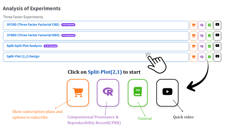
The module is reached from the RAISINS home page at www.raisins.live by way of the Data Analysis section, where it is listed as Split Plot (2,1).
5.1 Computational Provenance & Reproducibility Record
CPRR (Computational Provenance & Reproducibility Record) provides a transparent and comprehensive record. Selecting the CPRR icon beside the module gives access to the computational workflow performed during the analysis. The record for this module states the R version and the exact version of every package employed, and identifies the specific function underlying each reported result: the model that is fitted, the manner in which each error term is extracted, and the derivation of the critical differences and letter groupings. CPRR lists every default parameter and decision rule applied by the module and provides fully runnable R code reproducing each analytical step. Users can execute the code in R to independently reproduce and verify the results. It carries its own DOI.
For citation of the platform itself in a paper, thesis or report, the RAISINS citation is available in APA, Harvard and BibTeX formats at www.raisins.live/citation.html. This constitutes the primary reference and is sufficient for most manuscripts.
The CPRR for Split Plot (2,1) is available at www.raisins.live/module_record/splitplot21.html.
6 Preview mode and Quick Tour
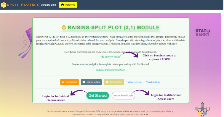
The module may be examined in full prior to subscription by means of Preview mode, accessible from the corresponding link on the Welcome page. An email address is entered, a one-time password is issued, and the whole of the module then becomes available: the complete analysis of variance, all seven tables of means, the entire graphical output and the RA-One assistant, operating upon the three datasets supplied with the module. No registration is required and no charge is made. The upload of user data is disabled in Preview mode.
A Quick Tour is additionally offered to first-time users, providing an interactive walkthrough of each control and its function. It may be repeated at any time from the Quick Tour tab in the navigation bar.
7 The worked example
The remainder of this tutorial employs Dataset 1, one of the three datasets supplied with the module (Section 8.3). It records a split-plot experiment comprising:
- Mainplot1 - main-plot factor 1, two levels (
A,B) - Mainplot2 - main-plot factor 2, two levels (
S1,S2) - Subplot - the sub-plot factor, two levels (
ss1,ss2) - Block - four replications
- Seven recorded characters,
YieldandChar1toChar6
Two levels of the first main-plot factor crossed with two levels of the second give four main plots per block, each subdivided into two sub plots for the two sub-plot levels; four blocks of eight sub plots yield 32 observations in total. Figure 1 illustrates the two-stage layout for a larger design; the principle is identical here, with four main plots to a block rather than six, and two sub plots within each rather than three.
The levels of the first main-plot factor are themselves named A and B. To keep them distinct from the factor labels A, B and C used in Section 2, level names are set in code font throughout.
A single character, Yield, is followed throughout. For a design of this size, the expressions of Section 3 give 9 degrees of freedom for Error(a) and 12 for Error(b); these are the figures to check against the ANOVA table once the analysis has been run (Section 10.1).
8 Preparation of the data file
The validity of any analysis is conditional upon the quality of the data submitted to it. Four routes to a correctly structured data file are available within the platform:
- Construction of the dataset in MS Excel
- Generation of the dataset within the RAISINS application
- Adoption of a supplied model dataset as a template
- Generation of the dataset through the RA-One chat assistant
8.1 Preparation in MS Excel
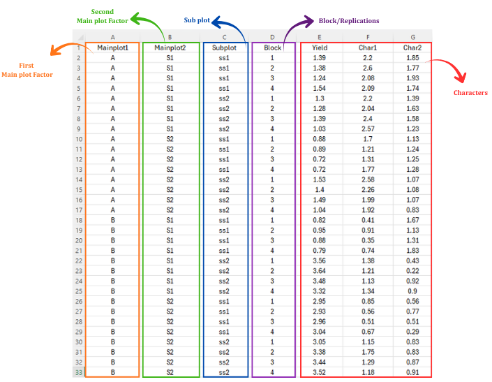
The module requires the data in long format: one row per observed sub plot, with the design recorded explicitly in columns rather than implied by the arrangement of the worksheet. A minimum of five columns is required:
| Column | Contents | Example values |
|---|---|---|
| Main plot factor 1 | Levels of the first main-plot factor | A, B |
| Main plot factor 2 | Levels of the second main-plot factor | S1, S2 |
| Sub plot | Levels of the sub-plot factor | ss1, ss2 |
| Block | Replication or block number | 1, 2, 3, 4 |
| One column per character | The recorded observations | 1.39, 2.20, … |
Column names may be chosen freely, since each column is assigned to its role after upload; Irrigation, Plough and fertilizer are therefore admissible. The structural requirements are as follows:
- One row per sub plot. For a 2 × 2 × 2 design in four blocks this gives 32 rows together with a header row.
- Every treatment combination present in every block, with no omissions.
- No blank cells, including no trailing blank rows or columns. These are detected on upload and the file is rejected.
- All characters recorded in adjacent columns. Any number may be analysed in a single run.
- The file saved in
.csvor.xlsxformat.
Level names should be brief and free of spaces (A1 in preference to Irrigation regime 1). They are reproduced as the row labels of every table of means and as the axis labels of every plot; extended names are the principal cause of illegible graphical output.
Dataset creation rules
- Column naming convention
- No spaces are permitted in column names.
- Use an underscore (
_) or a full stop (.) for separation. - Avoid symbols and special characters such as % and #.
- Data arrangement
- Begin the data at the upper-left corner of the sheet.
- Ensure the row immediately above the data is not blank.
- Keep the data on a single worksheet.
- Cell management
- Avoid typing in, or deleting from, cells outside the data region.
- Where such cells have been disturbed, select them, right-click and choose Clear Contents.
- Column relevance
- Name every column meaningfully.
- Exclude columns not required for the analysis.
- Factor levels
- Each of the two main-plot columns and the sub-plot column must contain exactly the intended number of distinct levels.
- Keep the spelling and capitalisation of every level consistent throughout its column.
- Balance
- Every A × B × C combination must appear once, and once only, in every block.
How to save as CSV in MS Excel
Open the workbook. Confirm that the data are arranged as described above and that the workbook contains a single sheet.
Select the ‘File’ menu at the top-left corner.
Choose ‘Save As’ or ‘Save a Copy’ and select the destination.
Set the file type to CSV. In the ‘Save as type’ list, choose CSV (Comma delimited) (*.csv).
Name the file, without spaces; an underscore may be used in their place.
Select ‘Save’ to export the file.
Before saving, verify once more that the data occupy the first sheet, that no blank row separates the header from the observations, and that the factor columns contain only the intended level names.
8.2 Generation using Create Data
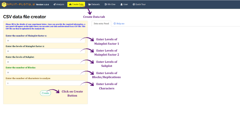
Where the data file is not to be constructed manually, the Create Data tab in the navigation bar generates a correctly structured, empty template. The following are specified:
- the number of levels of Mainplot factor 1,
- the number of levels of Mainplot factor 2,
- the number of levels of the Subplot factor,
- the number of Blocks, and
- the number of characters to analyse.
Selecting Create generates every row of the design, with the treatment and block columns completed and the character columns left blank, and provides the result as a CSV download. The observations are then entered in the blank columns and the file uploaded.
8.3 Model datasets
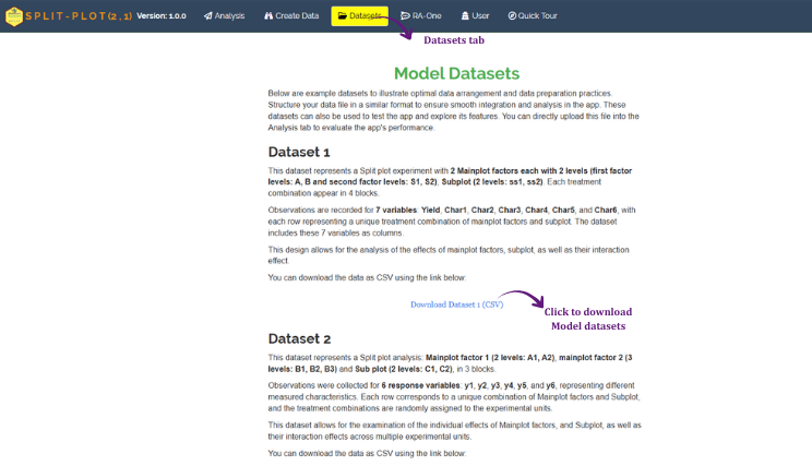
The Datasets tab provides three prepared Split Plot (2,1) datasets for download in CSV format. They serve both as structural templates and as a means of evaluating the module in advance of the user’s own data. Dataset 1 is that employed throughout this tutorial.
8.4 Generation through RA-One
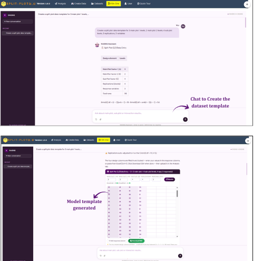
A template may also be requested directly of the assistant. In the RA-One tab, a request of the form “Create a split plot data template for 3 main plot 1 levels, 3 main plot 2 levels, 2 sub plot levels, 3 replications, 7 variables” causes the layout to be constructed, displayed in the chat and offered for download. The assistant additionally reports the degrees of freedom that the specified design leaves for Error(a), applying the minimum-replication criterion of Section 3, and issues a caution where that number is inadequate.
9 The Analysis tab
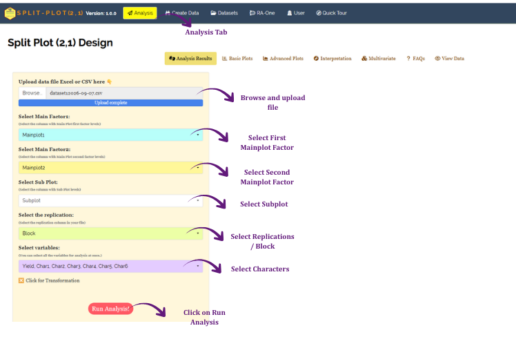
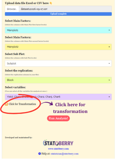
The module opens on the Analysis Results sub-tab, with the upload control and the variable selectors in the left-hand panel.
On upload, the file is validated for blank cells and for blank rows or columns, and the outcome reported. Five selectors are then presented in sequence, each highlighted in turn to indicate the next required entry:
- Select Main Factor1 - the column containing the first main-plot factor; for Dataset 1,
Mainplot1. - Select Main Factor2 - the second main-plot factor;
Mainplot2. - Select Sub Plot - the sub-plot factor;
Subplot. - Select the replication - the block column;
Block. - Select variables - the characters to be analysed. This selector admits multiple entries, and Select All submits every character in a single run.
Each selector withdraws its own selection from the remaining lists, so that no column may be assigned to two roles.
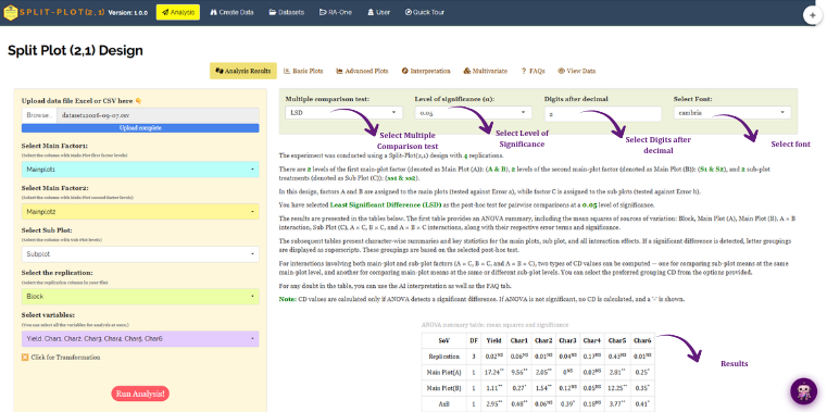
Selecting Submit executes the analysis and presents four settings above the results:
| Setting | Options | Function |
|---|---|---|
| Multiple comparison test | LSD (default), TUKEY, DMRT |
Determines the procedure used for mean separation and the resulting letter groupings (Section 4.1) |
| Level of significance (α) | 0.05 (default), 0.01 |
Threshold applied to both the F tests and the mean comparisons |
| Digits after decimal | 1 to 4 (default 2) | Rounding applied throughout the tabular output |
| Select Font | Cambria (default), Arial, Times New Roman, Helvetica, Courier New, Georgia, Verdana, Tahoma, Trebuchet MS | Typeface of the result tables |
9.1 Application of a transformation
The F tests assume that the residuals are approximately normal and that the error variance is homogeneous across treatments. Where a response is markedly skewed, or where its variance increases systematically with its mean, the Click for Transformation toggle below the selectors is enabled before the analysis is run. A panel then presents the Log option (for responses whose standard deviation is proportional to the mean), Square-root (for count data) and Arcsin (for proportions and percentages), and each character may be assigned to at most one of them. Where no assumption is violated, no transformation should be applied.
The analysis is thereafter performed on the transformed scale, and each table of means reports the transformed mean in parentheses beneath the original mean, so that the analysis remains traceable to the original observations. The data are validated before transformation: a square-root transformation applied to a column containing negative values, or an arcsine transformation applied to values outside the interval \([0, 1]\), is rejected with an explanatory message rather than being executed.
10 Analysis results
The output is presented as a sequence of tables. The first is a selection summary, confirming the role assigned to each column and the number of levels of each factor; it should be verified before the remaining output is examined (Figure 10).
10.1 The ANOVA table
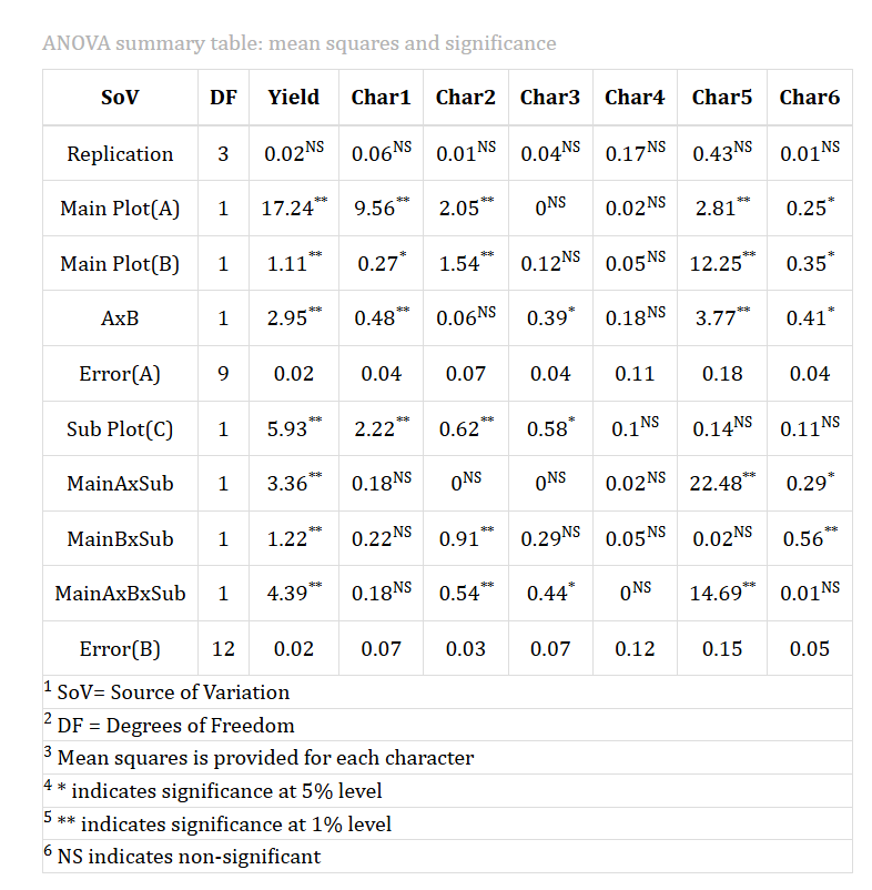
The analysis of variance is reported in ten rows, which reproduce the structure set out in Section 3. The first five constitute the main-plot stratum and terminate in Error(a); the last five constitute the sub-plot stratum and terminate in Error(b). Effects are flagged as significant at the 1 % level (**), at the 5 % level (*), or as non-significant (NS).
The analysis of variance obtained for Dataset 1 is shown in Figure 11, one column of mean squares for each of the seven characters.
Three features of the Yield column require attention.
The degrees of freedom correspond exactly to those derived in Section 7. Error(A) carries 9 and Error(B) 12. Where the reported degrees of freedom do not agree with the expressions of Section 3, the design specified to the module does not correspond to the design that was conducted, and the analysis should not be interpreted further until the discrepancy is resolved.
A × B is significant (mean square 2.95, flagged **; F = 121.53, p = 0.00 in the detailed table of Figure 13). By the rule of Section 3 this governs the interpretation of the two preceding rows: the effect of the first main-plot factor is conditional upon the level of the second with which it is combined, and its main-effect table does not constitute a complete account.
Every effect in the sub-plot stratum is significant, the three-factor interaction included. The sub-plot factor returns a mean square of 5.93 (**), and A × C (3.36), B × C (1.22) and A × B × C (4.39) are all flagged ** as well. The sub-plot effect is therefore not constant across the main-plot combinations, and by the rule of Section 3 it is the highest-order term - A × B × C - that governs the whole of the interpretation. The main-effect table for C records a real average difference, but it does not describe the behaviour of any particular combination, and the eight-cell A × B × C table (Figure 15) must be consulted before a recommendation is made.
The block effect is non-significant (0.02, NS), indicating comparative uniformity among the four replications. A significant block effect would not constitute a deficiency; it would indicate that blocking had removed a real source of variation.
How the F ratios of the table are formed
Each row’s F value is simply its own mean square divided by the mean square of the error term belonging to its stratum - for Yield, the main-plot effects (Main Plot A, Main Plot B, A × B) are each divided by Error(A) = 0.02, and the sub-plot effects (Sub Plot C, A × C, and so on) by Error(B) = 0.02. RAISINS makes this division automatically, so the important habit for the reader is simply to check, from the “Tested against” column of Section 3, that the right error term has been used for the effect in question.
For this character the two error mean squares happen to coincide at two decimal places (both 0.02), so the F ratios of the two strata are formed against divisors of much the same size. This is a coincidence of the data and not a property of the design: the two error terms are estimated independently of one another, and either can turn out the larger in a given experiment. What does differ between the strata, and always will, is the number of degrees of freedom carried by each - 9 against 12 - so that the same F value is judged against a different critical point in each stratum.
Significance is flagged with ** at the 1 % level and * at the 5 % level, NS denoting an effect not significant at the selected value of α.
10.2 Tables of means
A detailed table is reported for each of the seven effects. Each presents the treatment means with their letter grouping - means sharing a common letter do not differ significantly - followed by the supporting statistics of Section 4, each computed within that effect’s own error stratum, with one column per character:
| Row | Quantity |
|---|---|
| F stat, p value | The test for that effect, reproduced from the ANOVA |
| CD | Critical difference at the selected value of α |
| MSE(A) / MSE | The error mean square of the stratum against which the effect was tested |
| SE(m) | Standard error of a mean |
| SE(d) | Standard error of the difference between two means |
| CV(%) | Coefficient of variation of that stratum |
| Cohen’s F | Effect size, computed within that stratum (given for the main-effect tables) |
The two main-plot factors are both tested against Error(A), and the module reports them as shown in Figure 12. For Yield, the first main-plot factor gives 2.67 at level B (group a) against 1.20 at level A (group b), and the second gives 2.12 at S2 (group a) against 1.75 at S1 (group b), both with a critical difference of 0.12 and a coefficient of variation of 8.05 %.
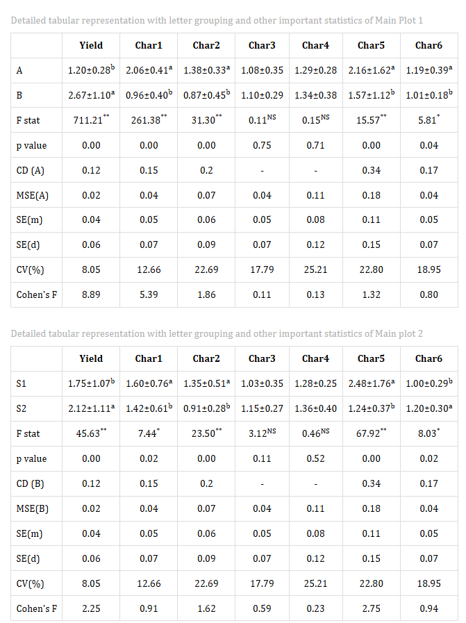
Considered in isolation these tables indicate that level B is the better of the two levels of the first main-plot factor, and S2 the better of the two levels of the second. Since A × B was significant, however, the interaction table must be examined before either conclusion is admitted. The module presents it as shown in Figure 13.
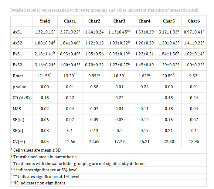
The main effect of the second main-plot factor makes S2 (2.12, group a) significantly superior to S1 (1.75, group b). The interaction table shows that this superiority is not merely unequal across the design but is actually reversed in one half of it. Under level B of the first factor the main-effect ordering holds and is substantial: BxS2 (3.16, group a) exceeds BxS1 (2.18, group b) by 0.98, far beyond the critical difference of 0.18. Under level A the ordering runs the other way: AxS1 (1.32, group c) exceeds AxS2 (1.08, group d) by 0.24, which likewise exceeds 0.18 and is therefore a real difference in the opposite direction.
An interaction of this kind - where the lines of a connected mean plot would actually cross rather than merely diverge - is the strongest form the rule of Section 3 can take. Recommending S2 on the evidence of its main effect alone would not simply overstate the advantage; it would give the wrong advice outright to anyone working under level A. The recommendation supported by the data is B in combination with S2, which records the highest combination mean in the experiment at 3.16, while S1 is the level to prefer wherever A is in use.
The sub-plot factor is tested against Error(B), and its table is shown in Figure 14.
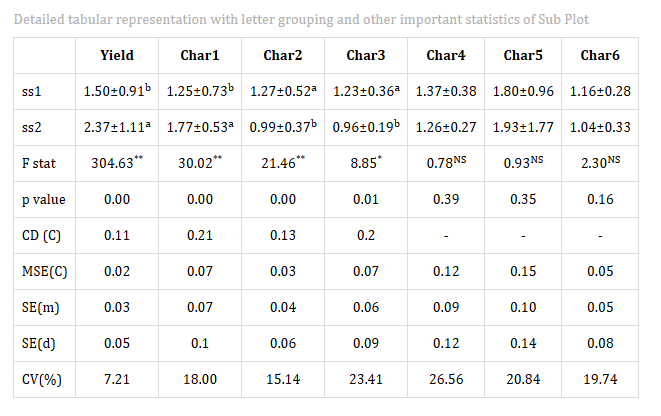
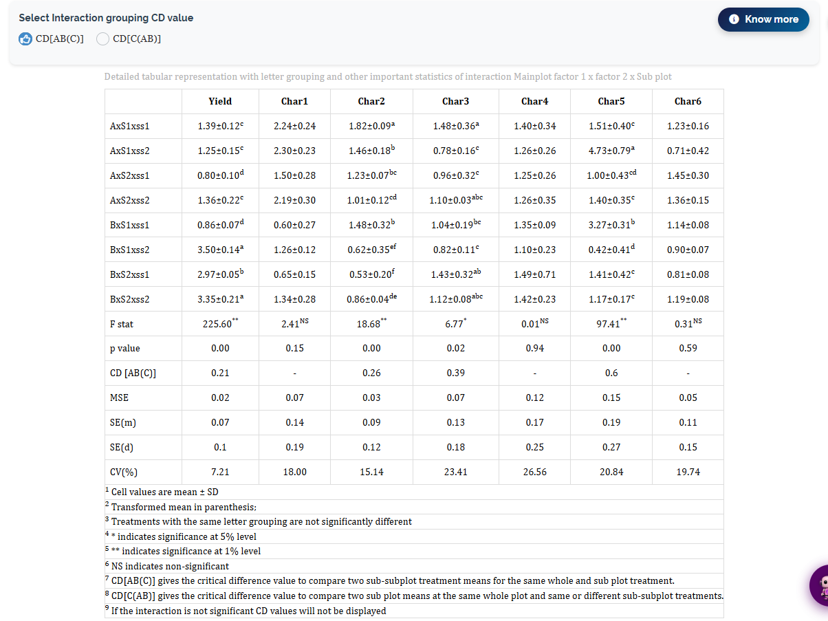
For Yield the difference between the two sub-plot levels is 0.87 - ss2 at 2.37 (group a) against ss1 at 1.50 (group b) - which greatly exceeds the critical difference of 0.11; ss2 is accordingly significantly superior on average. Because every interaction involving C attained significance, however, that average is not the end of the matter, and the A × B × C table of Figure 15 must be read before the difference is quoted for any particular treatment. Against its critical difference of 0.21, the advantage of ss2 is enormous under B with S1 (3.50, group a, against 0.86, group d), clear under B with S2 (3.35, group a, against 2.97, group b) and under A with S2 (1.36, group c, against 0.80, group d), but absent altogether under A with S1, where 1.25 and 1.39 share the group c and cannot be distinguished. The sub-plot main effect is thus a genuine average that describes no single cell of the design particularly well.
The two coefficients of variation differ - 8.05 % in the main-plot stratum and 7.21 % in the sub-plot stratum - each having been computed from its own error mean square as set out in Section 4. Both are reported, and both should be quoted with the stratum identified.
The effect sizes for this character are \(f = 8.89\) for the first main-plot factor and \(f = 2.25\) for the second. Both stand well above the 0.40 benchmark of Section 4.2, the first by a very wide margin: these are large effects and not merely statistically significant ones.
10.3 Interpretation of the worked example
Taken together, the seven tables tell a single coherent story about Yield, and it is a story in which no main effect can be quoted on its own. The main-plot stratum contributes a significant A × B interaction, so the two main-plot factors must be read as four combination means rather than as two separate rankings - the practical consequence being that the advantage of S2 over S1, clear enough in its own main-effect table, holds only under level B and is reversed under A. The sub-plot stratum then compounds this, every one of its terms being significant up to and including A × B × C: sub-plot level ss2 outperforms ss1 by a wide margin on average, but the size of that advantage varies from 2.64 under B with S1 down to nothing at all under A with S1.
The eight-cell A × B × C table is therefore the table to report, and the conclusion it supports is a single combination rather than a set of separate recommendations: B with S2 and ss2 (3.35) and B with S1 and ss2 (3.50) are the two highest means in the experiment, share the letter a, and cannot be separated from one another at α = 0.05; every other combination falls significantly below them. Where the main-plot factors are fixed by circumstance, the table also answers the narrower question directly - under A with S1, for instance, the choice of sub-plot level makes no difference at all.
A significant F test and a large effect size ordinarily go together, as they do here, but this need not always be so. An effect can be statistically significant yet modest in size where replication is generous, and conversely a genuinely large effect can fail to reach significance where replication is limited - a risk that is greatest for the main-plot factors, since Error(a) carries the fewest degrees of freedom in the design (Section 3). For this reason, the Cohen’s f column is worth reading alongside the p values rather than in place of them, and a non-significant result should be reported as inconclusive rather than as evidence that no effect exists.
10.4 Selection of the critical difference for cross-stratum comparisons
Where LSD has been selected as the comparison procedure and all factors have been assigned, the module presents additional controls above the interaction tables for selecting which of the two critical differences of Section 4 is applied to the letter grouping:
- CD[A(C)] or CD[C(A)] - comparison of first main-plot factor levels within a sub-plot level, or of sub-plot levels within a level of the first main-plot factor
- CD[B(C)] or CD[C(B)] - the corresponding pair for the second main-plot factor
- CD[AB(C)] or CD[C(AB)] - the corresponding pair for the A × B combinations
Each set is accompanied by a Know more control describing the comparison to which that critical difference applies. The selection must correspond to the comparison being reported.
The letter grouping shown automatically against the A × B, A × C, B × C and A × B × C tables is formed using the within-stratum critical difference - that is, CD[AB(C)] rather than CD[C(AB)], and correspondingly for the other two interactions. Where the comparison actually intended is the reverse - for instance, sub-plot levels compared across main-plot combinations rather than main-plot combinations compared within a sub-plot level - the corresponding radio button must be switched before the letters are read, since the default grouping does not answer that question.
10.5 Duncan’s multiple range test
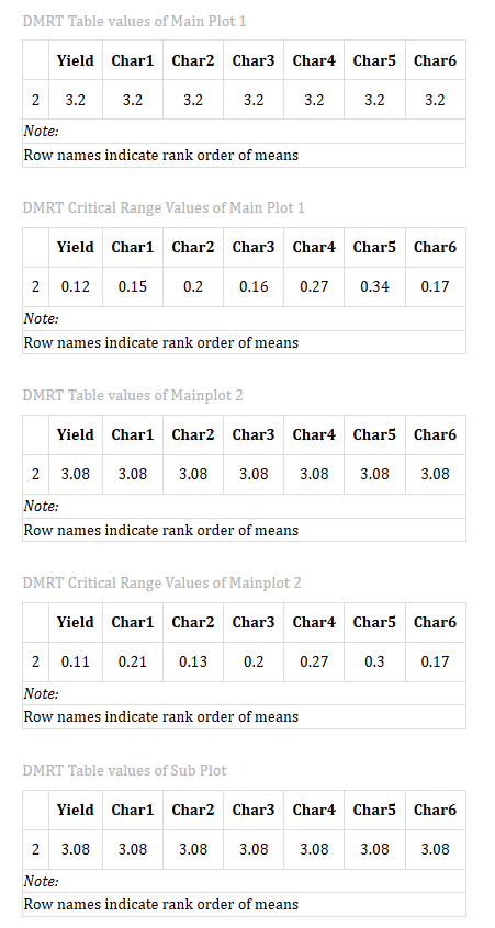
Where DMRT is selected, the module additionally reports for every effect a table of DMRT table values and a table of DMRT critical range values, giving the studentised range multipliers and the corresponding critical ranges at each span. Certain journals require these to be reported alongside the letter groupings.
10.6 Export of results
A Download report control below the tables provides the output in HTML, PDF or Word format. The selection summary, the analysis of variance and all tables of means are compiled into a single formatted document suitable for incorporation in a thesis chapter or for circulation. The Word format is appropriate where the tables are to be edited subsequently. Graphical output is downloaded individually from the respective plot tabs.
11 Basic Plots
The Basic Plots sub-tab provides five plot types:
- Boxplot - median, quartiles, whiskers and outliers for each treatment
- Violin Plot - the same distributional information rendered as a smoothed density
- Mean Value Plot - treatment means as points
- Connected Line Plot - means joined by lines
- Bar Plot - means as bars with error bars
Each plot carries a settings control providing a Plot Display Mode option - Faceted, presenting all selected characters in a single figure with the number of columns adjustable, or Individual, presenting one character at a time - together with controls for colours, themes, titles, axis labels, fonts, transparency and the display of grouping letters.
Each plot also carries a Select Factor control determining which effect is plotted on the abscissa. Six options are provided:
- Mainplot factor I (A)
- Mainplot factor II (B)
- Subplot factor (C) - the default
- Main I × Subplot (A × C)
- Main II × Subplot (B × C)
- Main I × Main II × Subplot (A × B × C)
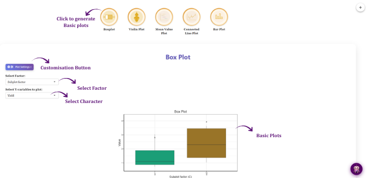
The Connected Line Plot is the standard representation: the sub-plot factor is plotted on the abscissa with one line per main-plot level, departure from parallelism indicating interaction. Main I × Subplot or Main II × Subplot is selected accordingly.
The A × B combination is not among the options provided. In the worked example, where A × B is one of the significant interactions, it cannot therefore be plotted from these tabs. RA-One should be used instead (Section 15), its in-chat plot toolbar including A × B among its effect options.
12 Advanced Plots
The Advanced Plots sub-tab provides ten further plot types:
| Plot | Purpose |
|---|---|
| Summary Plot | Box and bar representations combined in one figure |
| Raincloud Plot | Distribution, box and individual observations displayed together |
| Advanced Raincloud Plot | The same, with detailed control of the density, box and point layers |
| Circular Plot | All characters arranged radially for simultaneous comparison |
| QQ Plot | Assessment of residual normality |
| Distribution Plot | Ridge-style densities, one per treatment |
| Pair Plot | All pairwise scatterplots among the characters, with correlation coefficients |
| Correlation Plot | The correlation structure presented as a single graphic |
| 3D Scatter Plot | Three characters displayed simultaneously, rotatable |
| 3D Scatter + Line | The same, with a fitted line |
The Pair Plot carries its own Select Factor control, with the same six options as the Basic Plots. The QQ Plot provides the practical assessment of the normality assumption stated in Section 2.
A Q–Q plot ranks the residuals and plots them against the values that would be expected were they exactly normal. Where the assumption holds, the points lie close to the reference line. Gentle wandering about that line is of no consequence. A pronounced curve, a sigmoid, or points departing sharply at either extreme indicates a genuine departure from normality, and a transformation should then be considered (Section 9). Since a split plot carries two error strata, a departure should be referred to the stratum in which it arises: it bears upon the effects tested within that stratum, and not upon those tested in the other.
The module presents the relationships among the characters graphically only, through the Correlation Plot - a matrix of scatterplots with histograms on the diagonal and the correlation coefficients displayed in the upper panels - and the Pair Plot. No correlation results table is provided in the Analysis tabs.
Where the coefficients are required in tabular form for reporting or export, RA-One will produce the correlation matrix within the chat, with a Download CSV option (Section 15).
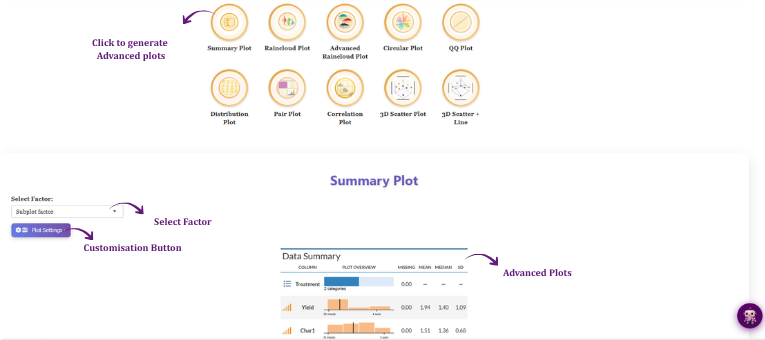
Where the number of treatment combinations is large, axis labels may overlap. The How to master Plots in RAISINS? guide, accessible from the plot tabs and from the FAQs, describes the available remedies: faceted display, adjustment of the number of columns, rotation of labels, abbreviation of level names and download at higher resolution.
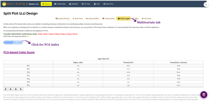
13 The Multivariate tab
Where several characters have been recorded, ranking treatments on each character separately may yield as many orderings as there are characters. The Multivariate sub-tab combines them into a single ranking by principal component analysis: the characters are standardised, decomposed into orthogonal components ordered by the variance they explain, and an index score is constructed from the leading component. The analysis is performed upon the means of the A × B × C treatment combinations for the selected characters, and requires at least two characters.
Selecting Click here for PCA Index produces, in order:
- an Eigen Values table, reporting the eigenvalue, the percentage of variance and the cumulative percentage for each component
- a Scree Plot of the eigenvalues
- a loadings table, giving the contribution of each character to each component
- a Biplot, representing treatments and character vectors upon the same axes
- an index score table and accompanying plot derived from PC1, and a corresponding pair derived from PC2
A cutoff for the scaled index is selected from the values 0.50, 0.75, 0.80, 0.90 and 0.95, the default being 0.75. Treatments falling on the selected side of this threshold are identified in the index tables and distinguished in the index plots. The module reports which components carry eigenvalues exceeding unity and issues a written caution where the first two components together account for less than 60 % of the total variation, in which case the index should be interpreted with caution. The index is exploratory: it yields a ranking, not a test of significance.
14 The Interpretation tab
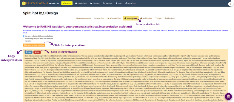
The Interpretation sub-tab renders the results as continuous prose. The confirmation box - “I’m not a robot and I have checked that on running analysis there was no error reported” - is ticked, whereupon a Click here for interpretation control appears. On selection, the assistant reads the analysis of variance and the tables of means and produces a paragraph-by-paragraph account, displayed progressively as it is generated.
The output is expressed in the terms of the experiment: which effects attained significance, the stratum against which each was tested, which treatments differed from which, and, where an interaction is significant, a statement that the main effects are not to be interpreted in isolation. It constitutes a first draft of a results section and a means of confirming that the tables have been read correctly.
Where the generated interpretation and the reader’s own reading of the tables diverge, one of the two is in error. Establishing which is considerably more informative than either account taken alone.
15 The RA-One assistant
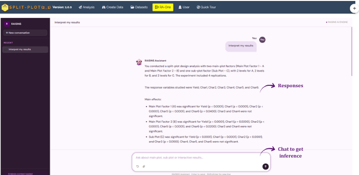
RA-One is the conversational assistant of the platform, available from the RA-One tab and from the chat control in the corner of the screen. Questions are posed in ordinary language and answered from the analysis that has been performed, rather than from generic statistical description. Every value reported is drawn from what the module computed; where a value is unavailable this is stated rather than inferred. Responses contain no code.
Once the results are loaded, four quick-start prompts are presented: Interpret results, addressing the main effects, the interactions and both error terms; Sub plot results, which opens the table of means for any of the seven effects; Model datasets, for retrieval of a supplied dataset; and Report results, for assistance in drafting the write-up. Questions may also be entered directly. A status indicator confirms that the analysis has been loaded into the conversation.
Within the Split Plot (2,1) module the assistant provides:
- Interpretation of the results, covering the main effects, the interactions and both error strata.
- Any of the seven tables of means. A request for the results table for A, B, C, A × B, A × C, B × C or A × B × C renders that table within the chat.
- The remaining result tables - the analysis of variance, the PCA eigenvalues, the loadings, the index scores derived from the first and second principal components, and the correlation matrix. The last of these merits particular note, being the sole result available in tabular form only through the assistant, the Analysis tabs presenting correlation graphically. Each card carries a Download CSV control.
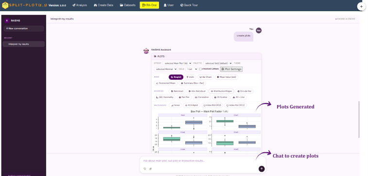
- Graphical output on request, rendered within the chat and restyled there. The available types comprise the box, violin, bar, mean value and connected mean plots; the summary, raincloud, distribution ridge and circular bar plots; the QQ, pair and correlation plots; the two three-dimensional plots; and the multivariate scree plot, PCA biplot and PC1 and PC2 index plots. Each carries its own toolbar, providing selection of the effect drawn, palette and theme, the number of columns, the display of grouping letters, a full settings panel and a download control. The effect selector of this toolbar includes A × B, which the module’s own plot tabs do not (Figure 22).
- Preparation of data, whether by construction of a template (Section 8.4) or retrieval of a supplied dataset (Section 8.3).
- Guidance on replication. Given a specified number of factor levels, the assistant applies the minimum-replication criterion of Section 3 to determine the minimum number of blocks maintaining Error(a) at twelve degrees of freedom or more, and reports the resulting Error(a) and Error(b) degrees of freedom together with the total number of experimental units. For the \(2 \times 2 \times 2\) design of the worked example the criterion calls for five blocks; Dataset 1 is replicated four times, and its Error(A) carries 9 degrees of freedom accordingly.
- Answers to questions of principle, concerning the structure of the design, the basis of the two error terms and the conventions governing the reporting of results.
RA-One is available to Institutional and Individual Full Licence subscribers.
16 FAQs
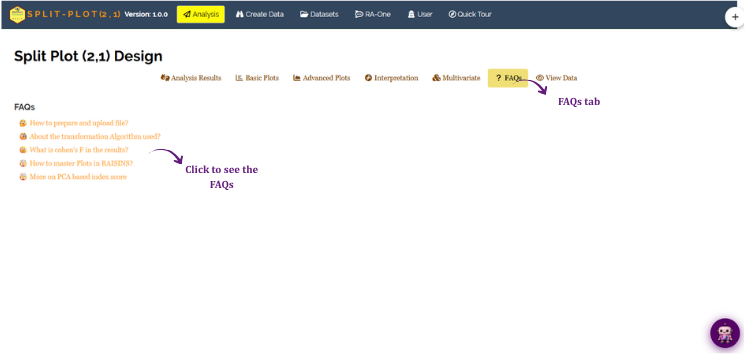
The FAQs sub-tab collects the extended guides of the module, each opening in its own panel:
- How to prepare and upload file?
- About the transformation Algorithm used?
- What is Cohen’s F in the results?
- How to master Plots in RAISINS?
- More on PCA based index score
These should be consulted where there is uncertainty as to the transformation to be applied, the interpretation of the effect-size column, or the presentation of a crowded plot.
17 View Data
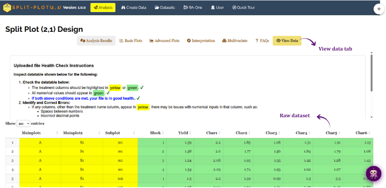
The View Data sub-tab displays the file exactly as the module has read it, together with the uploaded-file instructions, permitting verification of the data before the analysis is interpreted. Three checks should be made:
- The row count, which must equal the product of the numbers of levels of A, B and C and the number of blocks. For Dataset 1 this is 2 × 2 × 2 × 4 = 32.
- The level names, which should be examined for extraneous spaces and inconsistent capitalisation.
S1ands1are treated as distinct levels and will divide a single treatment into two without notification. - The absence of blank cells. Missing values are detected on upload and prevent the analysis from proceeding; this tab identifies their location.
18 Conclusion
The analysis of a Split Plot (2,1) design is based on a fundamental structural principle: because the treatments are randomised at two different plot sizes, the experiment involves two distinct error terms. Consequently, each treatment effect must be evaluated against its corresponding error stratum. The module automates this process by assigning the appropriate error terms and providing the associated standard errors, critical differences, and statistical letter groupings for each stratum.
Two important decisions, however, remain with the investigator. The first concerns the design stage, particularly the assignment of factors to the main plots and the selection of the number of blocks or replications. Since factors assigned to main plots are generally estimated with lower precision, the degrees of freedom associated with Error (a) can become limiting. These decisions should therefore be carefully considered before the experiment is established.
The second concerns the interpretation of treatment effects, particularly when interactions are significant. When a significant interaction is present, it should generally take precedence over the interpretation of the corresponding main effects. The worked example illustrates this clearly: although level S1 of the second factor shows a significantly higher main-effect mean, this advantage is observed only when combined with level A of the first factor and disappears under level B. Thus, interpreting the main effect alone would not adequately represent the treatment response.
If the experimental structure involves three successive levels of randomisation-main plot, sub-plot, and sub-sub plot-the Split-Split Plot module should be used. In contrast, when the experiment involves only two levels of randomisation-main plot and sub-plot-the Split Plot module is appropriate. If only one factor is assigned to the main plots without a sub-plot structure, the Split-Plot Design module should be used according to the experimental design.
For additional assistance, users can interact with RA-One, the integrated AI assistant, or contact the support team at [email protected].
