Three-Factor Factorial RBD
A three-factor factorial RBD tests three factors, their three two-way interactions and their three-way interaction in one blocked experiment, so that field or bench variation is removed from the error term. This tutorial explains the design, how to size it, and how to run and read the whole analysis in RAISINS… Read more …
A three-factor factorial Randomized Block Design (3F-RBD) allows three factors to be studied together in a single experiment. It shows the effect of each factor, how pairs of factors work together, and whether the effect of one factor changes according to the levels of the other two. Blocking is used to control known variation among experimental units, such as differences in soil, temperature, or experimental batches. This tutorial explains the design using a simple example, shows how to determine the number of treatment combinations and observations, and demonstrates how to analyse and interpret a 3F-RBD using RAISINS.
1 What is a three-factor factorial RBD?
Suppose you want to find out how fertilizer, irrigation, and variety affect crop yield. Instead of studying these factors one at a time, you can study them together in one experiment.
For example, consider:
- Fertilizer (A): F1, F2
- Irrigation (B): I1, I2, I3
- Variety (C): V1, V2
\[ 2 \times 3 \times 2 = 12 \]
different treatment combinations.
The important point is that the effect of one factor may depend on another factor. For example, a fertilizer may increase yield under high irrigation but have little effect under low irrigation. Similarly, one variety may respond well to a fertilizer while another variety may not. These are interactions, and a factorial experiment allows us to detect them.
If the field has a fertility gradient, we can divide it into similar blocks and place all 12 treatment combinations once in each block. The treatment combinations are then randomized within every block. This gives a three-factor factorial Randomized Block Design (3F-RBD).
In this design, we can answer three types of questions:
- Does fertilizer affect yield?
- Does the effect of fertilizer depend on irrigation or variety?
- Does the combination of fertilizer, irrigation, and variety produce a three-way interaction?
Does the effect of one factor depend on the levels of the others?
Factorial designs are used to study interactions between factors. The term “interaction” refers to how different factors work together to affect the outcome. In a factorial design, the second part of the name tells you how the treatment combinations are assigned to the experimental units. In a Randomized Block Design (RBD), also known as Randomized Complete Block Design (RCBD), you first group the experimental units into blocks. Each block contains units that are similar in some way. For example, you might group plants by soil type or group samples by the day they were collected. Once you have your blocks, you assign all 12 treatment combinations randomly within each block.
In a Completely Randomized Design (CRD), you can have unequal numbers of replicates for each treatment. This means that if you have more samples for one treatment than another, the analysis can still proceed. However, in a Randomized Block Design (RBD), this is not the case. In an RBD, each block must contain every treatment combination exactly once. This setup allows you to separate the effects of the blocks from the effects of the treatments.
In a three-factor factorial Randomized Block Design (RBD), you test three different factors at the same time. You do this within blocks of similar material to control for variation. This setup allows you to observe three main effects, the interaction between the factors and the three way interaction of all 3 factors.
2 How many observations will you need?
To size a three-factor factorial Randomized Block Design (RBD), you need two things. First, know how many levels each factor has. Second, determine the number of blocks.
- Let factor A have \(a\) levels, factor B have \(b\) levels and factor C have \(c\) levels.
- The number of distinct treatment combinations is the product
\[ a \times b \times c \]
- Each block holds all of them once, so with \(r\) blocks the total number of observations is
\[ N = a \times b \times c \times r \]
In this tutorial, you will work with a dataset that includes \(a = 2\), \(b = 3\), \(c = 2\), and \(r = 3\) blocks. These blocks result in \(2 \times 3 \times 2 = 12\) different treatment combinations. Overall, the dataset contains \(N = 12 \times 3 = 36\) observations.
In a Randomized Block Design (RBD), you allocate degrees of freedom to both treatments and blocks. This means you are considering two sources of variation. The error degrees of freedom are then calculated by subtracting the degrees of freedom used for treatments and blocks from the total degrees of freedom.
\[ df_{error} = (abc - 1)(r - 1) \]
In this experiment, you have \((12 - 1) \times (3 - 1) = 22\) error degrees of freedom. You will find this number in the Error row of the ANOVA table. The blocks in the experiment use \(r - 1 = 2\) degrees of freedom. In a Completely Randomized Design (CRD), these degrees of freedom would normally be part of the error. However, in this design, they are intentionally removed from the error. This helps prevent the error from becoming larger than necessary.
3 Main effects and interactions
In a three-factor experiment with blocks, you break down the variation into eight parts. These parts include seven treatment terms and one block term. Each part helps you answer a specific question about your experiment.
| Term | Degrees of freedom | The question it answers |
|---|---|---|
| Block | \(r-1\) | Did the blocks differ from one another, that is, was blocking worth doing? |
| A, B, C | \(a-1\), \(b-1\), \(c-1\) | Does this factor change the response, averaged over the other two? |
| A × B, A × C, B × C | \((a-1)(b-1)\), etc. | Does the effect of one factor depend on the level of the other, averaged over the third? |
| A × B × C | \((a-1)(b-1)(c-1)\) | Does the two-way interaction itself change from one level of the third factor to the next? |
The main effect of a factor is the change in the mean response as that factor moves from one level to another, averaged over every level of the other two factors. A two-way interaction measures the extent to which one factor’s effect is altered by another; if the two act independently, the interaction is zero and the two main effects tell the whole story. The three-way interaction is one step further: it asks whether the A × B pattern itself is different at level P1 of C than it is at P2. For the working example, \(a = 2\), \(b = 3\) and \(c = 2\), so the seven treatment terms carry \(1, 2, 1, 2, 1, 2\) and \(2\) degrees of freedom respectively, with 2 for blocks and 22 for error, exactly the layout of the ANOVA table in Section 9.
The Block row in your analysis is not about treatment effects. You do not report a “best block” because blocks are not treatments. Instead, this row helps you check if your local control was effective. When the block mean square is significant, it indicates that the material was indeed varied, and your design was useful. This means your blocking strategy successfully accounted for differences in the material. On the other hand, if the block mean square is not significant, it suggests that the blocks were similar. In this case, you have used two degrees of freedom without gaining any useful information. This is important to remember when planning your next trial, as it can help you decide whether blocking is necessary.
When you find that several terms in your analysis are significant, start by interpreting the highest-order significant term. For example, if the interaction between A, B, and C (A × B × C) is significant, this means that the effects of A, B, and C depend on each other in a complex way. In this case, the main effects and two-way interactions (like A × B or B × C) are averages that do not capture this complexity. Reporting only these averages could be misleading. Instead, you should focus on the cell means of the three-way table, as they provide a more accurate picture of the interactions. However, if the higher-order terms are not significant, then the main effects can fully summarise the experiment, as they reflect the overall trends without complex interactions.
4 Getting to the module
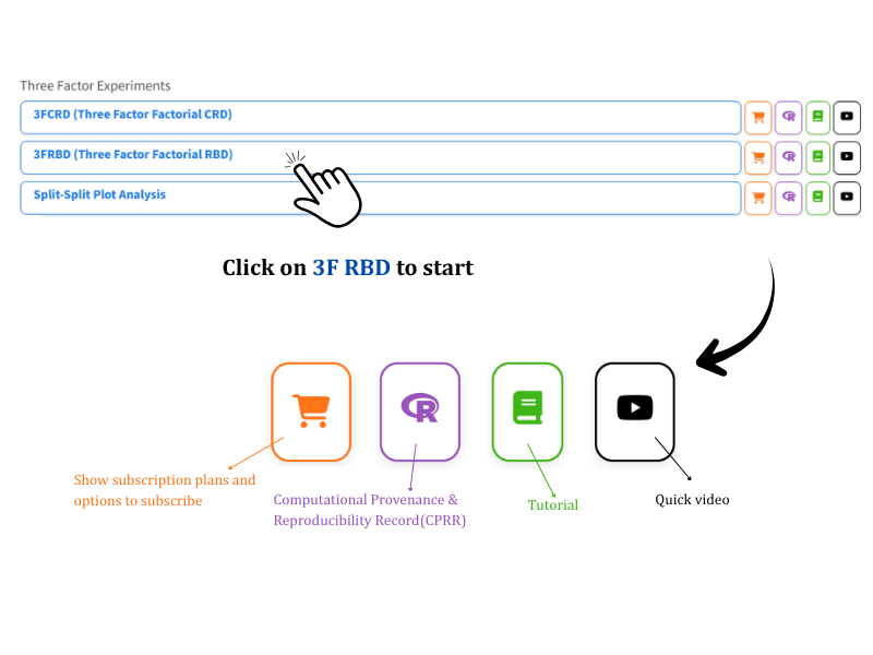
Go to the RAISINS home page at www.raisins.live. Open the Analysis of Experiment section. Here, you will find options for single-factor and multifactor experimental designs. Under Three Factor Experiments, select 3FRBD (Three Factor Factorial RBD) (Figure 1). You do not need to write any code for this. Simply upload your dataset. Then, choose the three columns that represent your factors, the column that represents the blocks, and the columns for your responses. The module will automatically generate all the necessary tables, plots, and interpretations for you. It will start on the Analysis Results tab, where you will see the upload panel ready for your data.
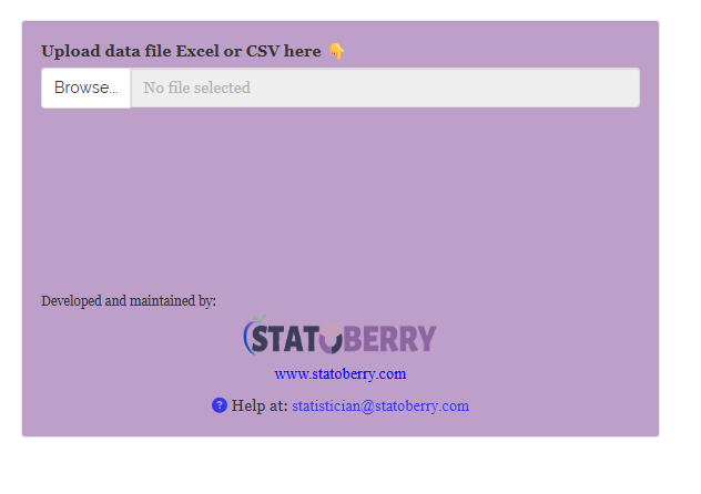
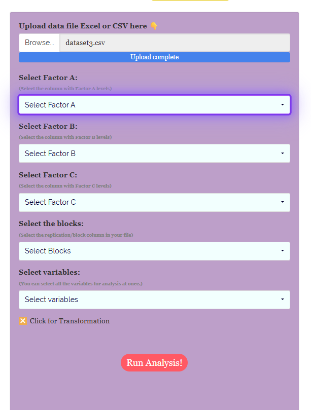
To begin, go to the Analysis tab (Figure 2) and upload your data. Once your data is uploaded, identify the correct columns that RAISINS should use for the analysis. After selecting the appropriate columns, click Run Analysis (Figure 3) to start the process.
4.1 Computational Provenance & Reproducibility Record
The CPRR (Computational Provenance & Reproducibility Record) gives you a clear and detailed account of the analysis process. To view this, click the CPRR icon located in the module header. This record shows the R version and the exact version of every package used in the analysis. It also names the specific function responsible for each result you see. CPRR includes a list of every default parameter and decision rule that the module applies. It also provides fully runnable R code that reproduces each analytical step. You can run this code in R to independently reproduce and verify the results. The record also has its own DOI, ensuring it is uniquely identifiable.
When you need to cite the platform in a paper, thesis, or report, use the RAISINS citation. You can find it in APA, Harvard, and BibTeX formats at www.raisins.live/citation.html. This citation serves as the main reference, and it is usually sufficient for most manuscripts.
You can find the CPRR for the three-factor factorial Randomized Block Design (RBD) module at www.raisins.live/module_record/3FRBD.html.
When you write a paper using the RAISINS platform, you should cite the RAISINS paper as your main reference. This gives credit to the platform and its developers. If a journal requires detailed information about the computing environment you used, or if you want to be specific about the versions and functions in your methods section, include the CPRR as supporting documentation. This is better than just saying “analysis was carried out using an online tool.” The CPRR further supports your citation and helps ensure that others can reproduce your computational results accurately.
5 Preview mode and Quick Tour
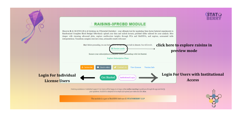
Before you subscribe, you can explore the entire module using Preview mode. You can access this mode from the Welcome page (Figure 4). In Preview mode, a built-in three-factor blocked dataset is loaded for you. This allows you to try out every feature without needing to upload your own file. You can experiment with the factorial ANOVA, which includes a block row, and explore post-hoc comparisons. You can also view interaction and diagnostic plots, as well as the MANOVA and PCA index. Additionally, the RA-One assistant is available for you to try. For first-time users, there is a Quick Tour. This is an interactive walkthrough that highlights each control and explains its function. You can retake the tour at any time by selecting the Quick Tour tab. This tab is located on the top navigation bar next to Analysis, Create Data, Datasets, RA-One, and User (Figure 8).
6 A working example
In this tutorial, you will work with a dataset shown in Figure 5. The dataset is structured as a three-factor factorial in a Randomized Block Design (RBD). It includes three factors: chemical1 as Factor A with 2 levels (S1, S2), chemical2 as Factor B with 3 levels (F1, F2, F3), and chemical3 as Factor C with 2 levels (P1, P2). This setup results in \(2 \times 3 \times 2 = 12\) different treatment combinations. These combinations are organised into 3 blocks (R1, R2, R3), with each block containing all 12 combinations once, leading to a total of \(N = 36\) observations. The dataset records eight traits, named char1–char8, but this tutorial focuses on analysing four of them: char1–char4. The first three columns of the dataset contain the labels for the three factors, the fourth column indicates the block, and the remaining columns contain the response data. The module will help you determine, for each character, whether it is influenced by chemical1, chemical2, chemical3, any pair of these chemicals, or all three together, while considering variations between blocks.
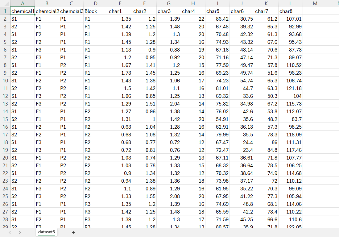
In this module’s demonstration file, there are two headers with typos: chemcial2 and chemcial3. They should be chemical2 and chemical3. These headers are shown exactly as they appear on the screen to ensure that the screenshots match the text. The application does not have an issue with this because a column name is just a label. What is important is that the label does not contain spaces and is spelled the same way throughout the column.
7 How to prepare your data
The quality of your analysis depends on the quality of your data. If you provide high-quality data, you will get reliable and insightful results. However, if your data is messy or inaccurate, the results will not be trustworthy. You have four options for handling your data:
- Create your dataset in MS Excel (Section 7.1)
- Build your dataset directly within the RAISINS app (Section 7.2)
- Use the Model dataset in RAISINS as a reference (Section 7.3)
- Create your dataset using the RA-One chat assistant (Section 7.4)
7.1 Preparing data in MS Excel
Start by organising your data file as described in Figure 5, with the role of each column marked in Figure 6. In the first column, enter the levels of Factor A. For example, if Factor A is chemical1, you will list its levels as S1 and S2. In the second column, input the levels of Factor B. If Factor B is chemcial2, its levels might be F1, F2, and F3. The third column should contain the levels of Factor C. If Factor C is chemcial3, its levels could be P1 and P2. The fourth column is for the block or replication label. If this is Block, you will use levels R1, R2, and R3. Each additional column represents a response variable, such as char1, char2, and so on. Each row in your file corresponds to one experimental unit. For instance, if you have 12 combinations and 3 blocks, your file will have 36 rows. Ensure that you spell each level label consistently and do not leave any blank rows above or within your data. Once your data is correctly laid out, save the file as a CSV before uploading it.
When you are working with this method, it is crucial to ensure that every block includes every treatment combination exactly once. This is stricter than in a Completely Randomized Design (CRD). Every block must hold the full set of combinations, one row each, so with 12 treatment combinations each block must have exactly 12 rows. Before you save your work, sort your data sheet by block. Then, check that each block indeed contains all 12 rows. This step ensures that your data is complete and correctly organised for analysis.
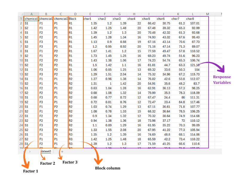
char1 onward is a response variable. This is the layout RAISINS expects, and the order matters: the three factors first, the block fourth, the responses last
Dataset creation rules
- Column naming convention
- No spaces allowed in column names.
- Use underscores (
_) or full stops (.) for separation. - Avoid symbols and special characters such as %, #.
- Data arrangement
- Start the data towards the upper-left corner.
- Ensure the row above the data is not blank.
- Cell management
- Avoid typing or deleting in cells without data.
- If needed, select the affected cells, right-click, and choose Clear Contents.
- Factor, block and response columns
- The first three columns must be the three factors (factorA, factorB, factorC), the fourth the block column, and every remaining column a numeric response.
- Use the same label for a level everywhere it appears, so RAISINS reads the correct number of levels.
- Blocking
- Enter one row per experimental unit; do not average blocks into a single row.
- Each block must contain every treatment combination exactly once. Unlike a CRD, an RBD does not tolerate a missing or a duplicated combination within a block.
How to save as CSV in MS Excel
Open your workbook. Ensure your data is arranged properly with only one sheet.
Click the File menu. Go to the top-left corner and click File.
Choose Save As or Save a Copy. Select the location where you want to save your file.
Set file type to CSV. In the Save as type dropdown, choose CSV (Comma delimited) (*.csv).
Name your file. Enter a relevant file name without spaces (use underscores if needed).
Click Save. Click Save to export the file.
💡 Tip: Before saving, double-check that your data is on the first sheet and follows the required format.
7.2 Prepare using Create Data in RAISINS
To set up your data correctly, you can use the application to create the layout for you. Start by opening the Create Data tab (Figure 7). Here, you need to enter several pieces of information: the number of levels for Factor A, Factor B, and Factor C, the number of Blocks, and the number of response columns you need. Once you have entered these details, click Create. This action will populate the data-entry panel on the right with all possible treatment combinations. Each combination will appear once for each block, and the response columns will be empty, ready for you to input your data (Figure 7). You can either type the values directly into these columns or paste data from Excel using Ctrl + V. After entering your data, click Download CSV file. You will then need to upload this file under the Analysis tab to proceed with your analysis.
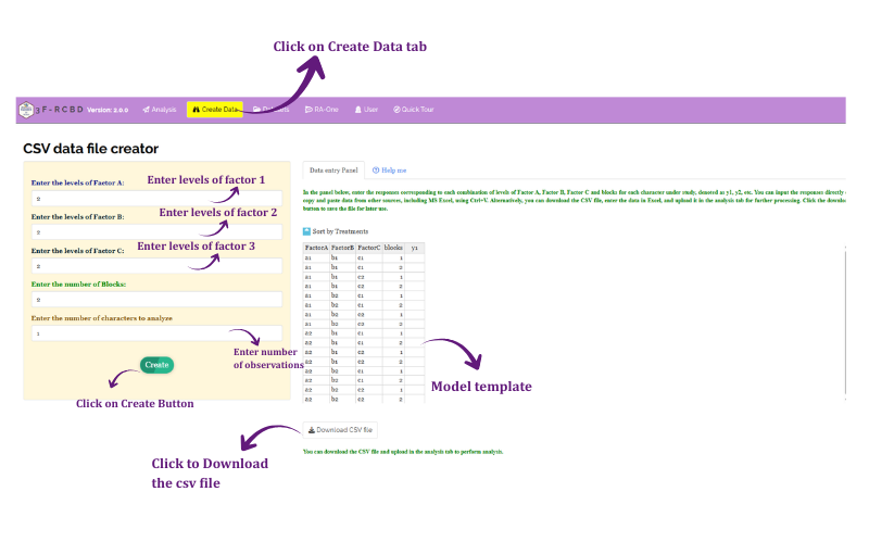
y1 column left empty for your readings. Download CSV file saves the completed sheet for upload under the Analysis tab
7.3 Download the Model dataset
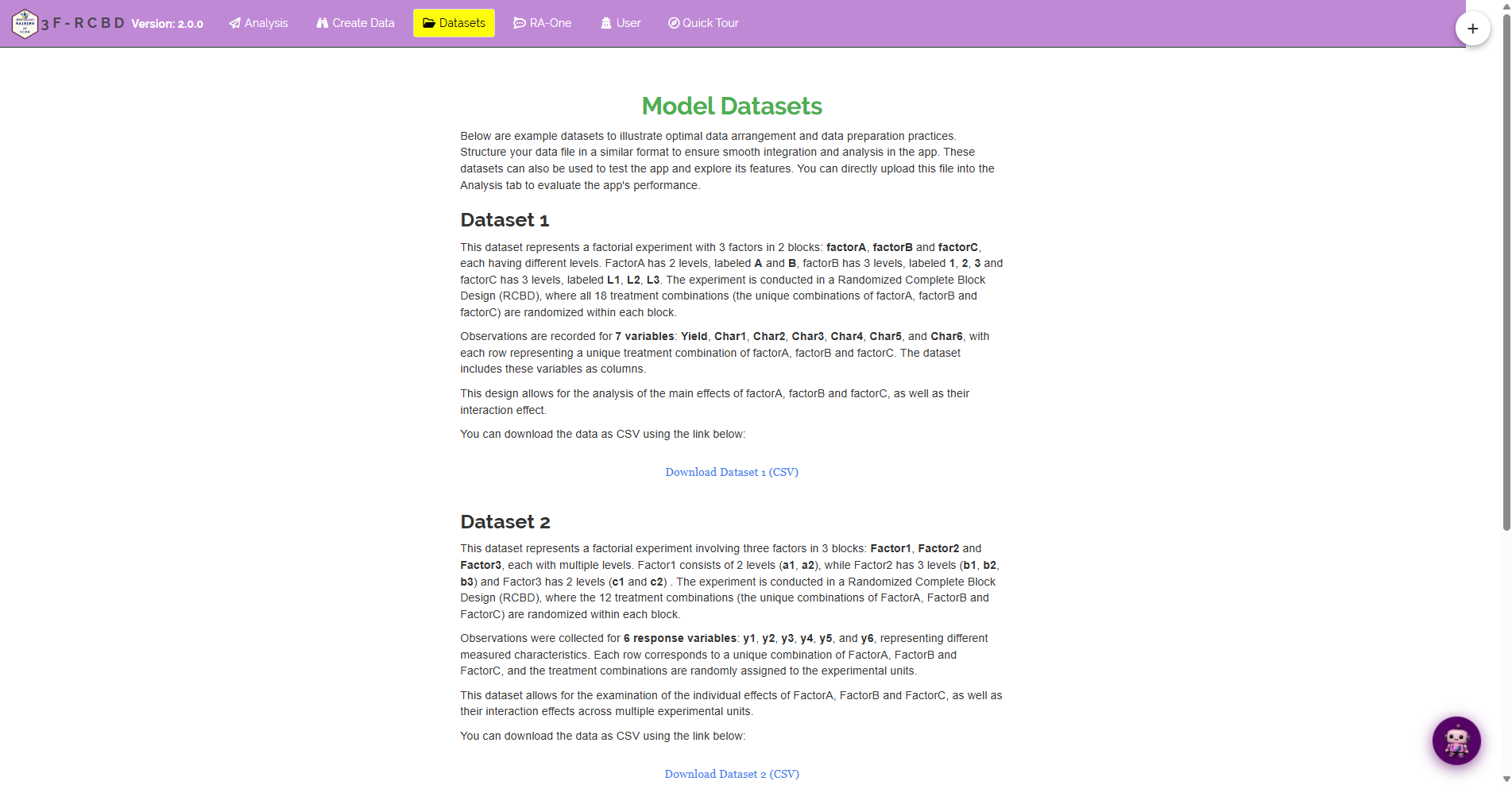
If you want to try out the module before using your own data, you can use the model datasets (Figure 8) provided. To do this:
- Open the Datasets tab
- Read the description of each dataset and click its Download CSV link
- Save the file, then either study its layout as a reference for your own file or upload it directly under Analysis to see the full analysis at once
Dataset 1 consists of a factorial design with 2 levels for the first factor, 3 levels for the second, and 3 levels for the third, arranged in 2 blocks. This results in 18 different treatment combinations. It includes seven variables. Dataset 2 has a factorial design with 2 levels for the first factor, 3 levels for the second, and 2 levels for the third, arranged in 3 blocks. This results in 12 treatment combinations and includes six response variables. It matches the shape of the working example in this tutorial.
7.4 Creating a dataset using RA-One chat
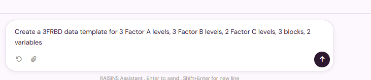
The built-in chat assistant, RA-One (Section 14), helps you create a correctly formatted template through a simple conversation. You describe your experiment in words. For example, you might say, “Create a 3FRBD data template for 3 Factor A levels, 3 Factor B levels, 2 Factor C levels, 3 blocks, 2 variables” (Figure 9). The assistant then provides you with a ready-to-fill table (Figure 10). This table includes the error degrees of freedom, which allows you to assess if your design has enough power before you start collecting data. Once you have the table, fill in your responses, download the CSV file, and upload it under the Analysis tab. You can do all of this without leaving the chat.
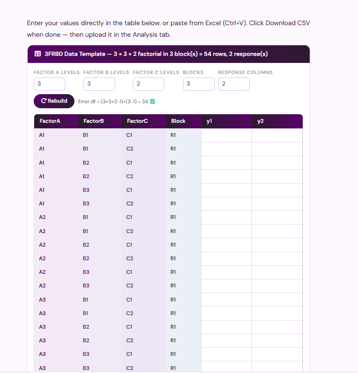
y1 and y2 columns, or paste them from Excel with Ctrl + V, then click Download CSV and upload the file under the Analysis tab
8 The Analysis tab
Once your CSV file is ready, go to the Analysis tab. Click on Browse… under the section labeled Upload data file Excel or CSV here and choose your file (Figure 2). You will see a blue Upload complete bar, which confirms that your file has been successfully loaded. The application will then read the column names from your file. It will prompt you to identify the correct columns (Figure 3) for your analysis.
- Select Factor A - the column holding the levels of the first factor (here,
chemical1). - Select Factor B - the column holding the levels of the second factor (here,
chemcial2). - Select Factor C - the column holding the levels of the third factor (here,
chemcial3). - Select the blocks - the replication or block column (here,
Block). This picker is the one control that does not exist in the CRD module, and getting it right is what allows the block row to appear in the ANOVA. - Select variables - one or more response columns to analyse; you may select several at once (here
char1–char4), and RAISINS analyses each in turn. - Click for Transformation - an optional toggle to transform a skewed response before analysis.
Once you have selected the columns you want to analyse, click the “Run Analysis” button. This action applies a full factorial model with a block term to each response you have chosen. The results are organised into several sub-tabs for easy access. These sub-tabs include “Analysis Results”, where you can see the outcomes of the analysis, and “Summary stats”, which provides basic statistical summaries. “Individual ANOVA” shows the analysis of variance for each response. “Basic Plots” and “Advanced Plots” offer visual representations of the data. “Interpretation” helps you understand the results, while “Multivariate” deals with analyses involving multiple variables. “FAQs” provides answers to common questions, and “View Data” lets you look at the raw data.
When you analyse your data, you do not need to run the module separately for each response. Instead, select all the response columns at once. This way, the software generates a complete set of tables for you. These include an ANOVA table, a mean-comparison table, and an effect-size table for each response column. Additionally, it produces a single MANOVA table that covers all the response columns together. This is why, in the next section, you will see results tables with one column for each trait, labelled char1 to char4.
8.1 Optional: transforming a response
In factorial ANOVA, you assume that the response variable follows a normal distribution and that the variability is similar across different treatments. This means that the data should look like a bell curve and have a similar spread for each group you are comparing. However, if the data is not like this, for example, if it is skewed or if the spread increases as the mean increases, you need to transform the data before analysing it. To do this, click Click for Transformation and select a suitable transformation. This step is important because it helps make the data fit the assumptions of the ANOVA. The application provides three standard transformation options and makes necessary adjustments for any unusual values to ensure the analysis is accurate.
| Transformation | Use it when | What RAISINS applies |
|---|---|---|
| Logarithmic | The spread grows in proportion to the mean (multiplicative data) | \(\log_{10}(x)\); if any value is \(\le 0\), it shifts first as \(\log_{10}(x - \min + 1)\) |
| Square-root | Counts, or data following a Poisson-like pattern | \(\sqrt{x}\); if any value is \(0\), it uses \(\sqrt{x + 0.5}\); negative values are not allowed |
| Arcsine | Proportions or percentages between 0 and 1 | \(\arcsin(\sqrt{x})\), with \(0\) and \(1\) nudged by \(1/(4n)\) so the transform stays finite |
When you apply a transformation, you temporarily change the scale of your data to make the statistical test valid. This does not alter your actual experiment. Always report that you used a transformation, but when discussing results, use the original units for means and recommendations. If your data meets all assumptions, do not apply a transformation. Unnecessary transformations can make your results more difficult to understand. To quickly check if a transformation is needed, use the QQ plot in Section 11.
9 Analysis results
The Analysis Results sub-tab displays the factorial ANOVA. A control strip at the top allows selection of the multiple-comparison test (default is LSD, with options for Tukey’s HSD and Duncan’s DMRT), level of significance (\(\alpha\), default is 0.05), digits after decimal, and font. Below, a paragraph summarises the analysed experiment, followed by eight tables: the ANOVA summary, one table for each of the three factors, one for each of the three two-way interactions, and one for the three-way interaction. Each table includes one column per response (char1–char4).
Table 1: ANOVA summary - mean squares and significance
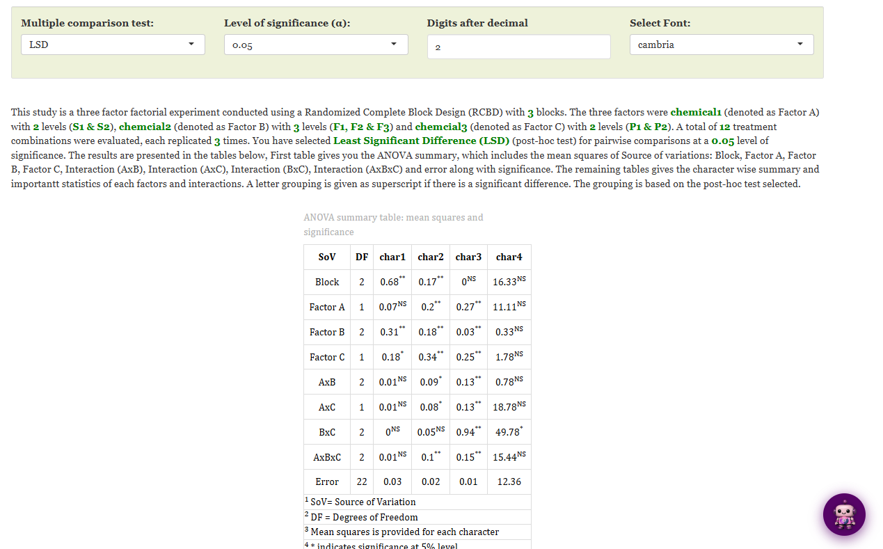
Each row represents a source of variation: Block (2 df), Factor A (1 df), Factor B (2 df), Factor C (1 df), A × B (2 df), A × C (1 df), B × C (2 df), A × B × C (2 df), and Error (22 df), aligning with the degrees of freedom predicted in Section 2 and Section 3 for a \(2 \times 3 \times 2\) experiment in three blocks. Each cell shows the source’s mean square for the response, with a superscript flag: * for significance at 5%, ** at 1%, and NS for non-significant.
The Block row is significant for char1 (\(0.68^{**}\)) and char2 (\(0.17^{**}\)), indicating genuine differences among blocks, leading to a smaller error and more precise treatment tests. It is non-significant for char3 (\(0^{NS}\)) and char4 (\(16.33^{NS}\)). In a CRD, block variation would have been included in the error.
The treatment rows reveal four distinct patterns. char1 is influenced by Factor B (\(0.31^{**}\)) and Factor C (\(0.18^{*}\)), with Factor A and all interactions non-significant, making it the simplest case. char2 is affected by all three main effects (A \(0.2^{**}\), B \(0.18^{**}\), C \(0.34^{**}\)), the interactions A × B (\(0.09^{*}\)) and A × C (\(0.08^{*}\)), and the three-way A × B × C (\(0.1^{**}\)). char3 shows significance in all seven treatment terms, with the largest effect being B × C at \(0.94^{**}\). char4 is unexpected: all three main effects and the three-way interaction are non-significant, but B × C is significant at \(49.78^{*}\). Each significant term is detailed in the subsequent tables.
Let’s focus on char4. When you look at Factor B (\(0.33^{NS}\)) and Factor C (\(1.78^{NS}\)) individually, they seem to have no effect on char4. If you only consider these main effects, you might think the experiment found no impact on char4. However, the B × C interaction row tells a different story. Here, Factors B and C influence char4 in opposite ways, depending on each other. This means that when you average over one factor, it cancels out the effect of the other, leaving the main-effect table with no visible result. This is a key reason for using a factorial design: it can detect interactions between factors that a one-factor-at-a-time experiment would miss.
How this table is built
RAISINS fits the linear model response ~ Block + A * B * C for each trait, which expands to the block term, the three main effects, the three two-way interactions and the three-way interaction, and forms the analysis-of-variance table from it. Each source’s mean square is its sum of squares divided by its degrees of freedom, and the F-test divides each treatment mean square by the error mean square; the p-value behind each F decides the * / ** / NS flag against the chosen \(\alpha\). Because the block term takes 2 of the 35 total degrees of freedom and the seven treatment terms take 11 between them, the error is left with 22, which is the figure \((abc-1)(r-1)\) predicts.
Table 2: Factor A - means and comparison statistics
This table shows the main effect of Factor A, averaged over Factor B, Factor C, and the blocks, across its two levels.
| Factor A | char1 | char2 | char3 | char4 |
|---|---|---|---|---|
| S1 | 1.20 ± 0.29 | 1.09 ± 0.24 | 1.19 ± 0.19 | 15.94 ± 3.49 |
| S2 | 1.29 ± 0.29 | 1.24 ± 0.25 | 1.36 ± 0.37 | 17.06 ± 3.84 |
| F stat | 2.24NS | 10.74** | 43.99** | 0.90NS |
| p value | 0.15 | 0.00 | 0.00 | 0.35 |
| CD (A) | – | 0.09 | 0.05 | – |
| MSE | 0.03 | 0.02 | 0.01 | 12.36 |
| SE(m) | 0.04 | 0.03 | 0.02 | 0.83 |
| SE(d) | 0.06 | 0.05 | 0.03 | 1.17 |
| CV(%) | 14.02 | 11.79 | 6.08 | 21.31 |
| Cohen’s F | 0.32 | 0.70 | 1.41 | 0.20 |
Factor A affects two of the four traits. For char2, \(F = 10.74^{**}\) (\(p = 0.00\)) with CD (A) \(= 0.09\): S2 (\(1.24 \pm 0.25\)) stands above S1 (\(1.09 \pm 0.24\)), and the gap of 0.15 exceeds the critical difference. For char3, the same ordering holds more emphatically, \(F = 43.99^{**}\) with CD \(= 0.05\) against a gap of 0.17, and a Cohen’s F of 1.41, indicating a very large effect. For char1 (\(2.24^{NS}\)) and char4 (\(0.90^{NS}\)), the F-statistic is non-significant, so the CD row reads “–”: RAISINS withholds the post-hoc yardstick when there is nothing to separate. The lower rows report the pooled MSE, the standard error of a mean SE(m) and of a difference SE(d), the coefficient of variation CV(%), and the Cohen’s F effect size. Note the low CV for char3 (6.08%) and the high CV for char4 (21.31%), hinting at why char4 shows so little.
Table 3: Factor B - means and comparison statistics
| Factor B | char1 | char2 | char3 | char4 |
|---|---|---|---|---|
| F1 | 1.42 ± 0.24 | 1.18 ± 0.25 | 1.34 ± 0.10 | 16.33 ± 2.99 |
| F2 | 1.22 ± 0.33 | 1.28 ± 0.13 | 1.24 ± 0.12 | 16.67 ± 3.39 |
| F3 | 1.10 ± 0.21 | 1.04 ± 0.30 | 1.25 ± 0.52 | 16.50 ± 4.70 |
| F stat | 10.20** | 9.73** | 5.70** | 0.03NS |
| p value | 0.00 | 0.00 | 0.01 | 0.97 |
| CD (B) | 0.15 | 0.12 | 0.07 | – |
| MSE | 0.03 | 0.02 | 0.01 | 12.36 |
| SE(m) | 0.05 | 0.04 | 0.02 | 1.02 |
| SE(d) | 0.07 | 0.06 | 0.03 | 1.44 |
| CV(%) | 14.02 | 11.79 | 6.08 | 21.31 |
| Cohen’s F | 0.96 | 0.94 | 0.72 | 0.05 |
Averaging over Factors A and C shows the main effect of Factor B, which is significant for three traits, with varying rankings. For char1, \(F = 10.20^{**}\) with CD (B) \(= 0.15\): F1 is highest at \(1.42 \pm 0.24\), outperforming F2 (gap 0.20) and F3 (gap 0.32), while F2 and F3 differ by only 0.12 and are on par. For char2, \(F = 9.73^{**}\) with CD \(= 0.12\): F2 leads at \(1.28 \pm 0.13\), but its margin over F1 is only 0.10, not clearing the CD; F3 (\(1.04 \pm 0.30\)) is below both. For char3, \(F = 5.70^{**}\) with a tight CD of \(0.07\): F1 (\(1.34 \pm 0.10\)) is above F2 (\(1.24\)) and F3 (\(1.25\)), which are indistinguishable. For char4, nothing separates (\(0.03^{NS}\)). Thus, the level of Factor B that maximises char1 and char3 does not maximise char2.
Table 4: Factor C - means and comparison statistics
| Factor C | char1 | char2 | char3 | char4 |
|---|---|---|---|---|
| P1 | 1.18 ± 0.29 | 1.07 ± 0.17 | 1.19 ± 0.26 | 16.28 ± 3.37 |
| P2 | 1.32 ± 0.28 | 1.26 ± 0.29 | 1.36 ± 0.33 | 16.72 ± 4.01 |
| F stat | 6.00* | 18.05** | 40.64** | 0.14NS |
| p value | 0.02 | 0.00 | 0.00 | 0.71 |
| CD (C) | 0.12 | 0.09 | 0.05 | – |
| MSE | 0.03 | 0.02 | 0.01 | 12.36 |
| SE(m) | 0.04 | 0.03 | 0.02 | 0.83 |
| SE(d) | 0.06 | 0.05 | 0.03 | 1.17 |
| CV(%) | 14.02 | 11.79 | 6.08 | 21.31 |
| Cohen’s F | 0.52 | 0.91 | 1.36 | 0.08 |
Factor C has two levels, so its F-test compares them. P2 is above P1 for all three significant traits: char1 (\(1.32\) against \(1.18\), \(F = 6.00^{*}\), CD \(= 0.12\)), char2 (\(1.26\) against \(1.07\), \(F = 18.05^{**}\), CD \(= 0.09\)), and char3 (\(1.36\) against \(1.19\), \(F = 40.64^{**}\), CD \(= 0.05\)). Char4 remains unchanged (\(0.14^{NS}\)). This is the most consistent main effect in the experiment, but interaction tables must be read first.
Tables 5–7: the two-way interactions
Three tables present the level combinations of each factor pair, averaged over the third factor and blocks, as mean ± SD. Letter groupings indicate significant interactions. They are summarised here.
Table 5, A × B shows significant interactions for char2 (\(F = 4.94^{*}\), CD \(= 0.16\)) and char3 (\(F = 22.15^{**}\), CD \(= 0.09\), Cohen’s F 1.42). The char3 column indicates the clearest interaction: under S1, the order of B levels is F1 (\(1.31\)) > F2 (\(1.22\)) > F3 (\(1.04\)), with F3 as the worst. Under S2, the order reverses, making F3 (\(1.46\)) the best, followed by F1 (\(1.37\)) and F2 (\(1.26\)). The lines cross, preventing any statement about “the best level of Factor B” without specifying the level of Factor A.
Table 6, A × C is significant for char2 (\(F = 4.46^{*}\), CD \(= 0.13\)) and char3 (\(F = 21.69^{**}\), CD \(= 0.08\)). The interaction is of magnitude rather than order. Moving from P1 to P2 increases char3 by \(0.04\) under S1 (\(1.17 \rightarrow 1.21\)) and by \(0.29\) under S2 (\(1.22 \rightarrow 1.51\)). Factor C is beneficial in both cases, but its effect is about seven times greater when Factor A is at S2. A similar pattern is observed in char2, with P1 to P2 increasing by \(0.10\) under S1 and \(0.30\) under S2.
Table 7, B × C is significant for char3 (\(F = 156.12^{**}\), CD \(= 0.09\), Cohen’s F 3.77, the largest effect in this analysis) and is the only significant source for char4 (\(F = 4.03^{*}\), CD \(= 4.21\)). For char3, moving from P1 to P2 lowers the response at F1 (\(1.42 \rightarrow 1.25\)) and F2 (\(1.31 \rightarrow 1.17\)), but nearly doubles it at F3 (\(0.85 \rightarrow 1.66\)). For char4, a similar pattern occurs: F1 decreases from \(18.33\) to \(14.33\), while F3 increases from \(14.50\) to \(18.50\), with a swing of \(4.00\) in each direction against a CD of \(4.21\). Both main effects disappeared because the movements cancel when averaged.
Table 8: the three-way interaction A × B × C
The last table has twelve rows, each representing a treatment combination (S1×F1×P1, S1×F1×P2, S1×F2×P1, …, S2×F3×P2). This detailed design is significant for two traits: char2 (\(F = 5.27^{**}\), CD \(= 0.23\), Cohen’s F 0.69) and char3 (\(F = 24.18^{**}\), CD \(= 0.13\), Cohen’s F 1.48). For char1 (\(0.24^{NS}\)) and char4 (\(1.25^{NS}\)), it is non-significant, so those columns have no letters.
S2×F3×P2 is the highest combination for char3 at \(2.05 \pm 0.02\), exceeding its nearest rival by \(0.5\) and surpassing the CD of \(0.13\). It is also the highest for char2 at \(1.52 \pm 0.02\). The lowest combination for both traits is S1×F3×P1, at \(0.83 \pm 0.09\) for char3 and \(0.86 \pm 0.08\) for char2. F3 appears at both extremes: with S1 and P1, it is the worst combination, and with S2 and P2, it is the best. This finding is not evident from any main-effect table and is the most important in this dataset.
Reading every row of the factor and interaction tables
- Mean ± SD - the level (or cell) mean and its standard deviation; a transformed mean, if a transformation was applied, is shown in parentheses.
- F stat / p value - the F-test for that source and its probability; the superscript (
*,**,NS) marks significance at the chosen \(\alpha\). - CD - the critical difference from the selected post-hoc test; two means differing by more than the CD are significantly different. Shown as “–” when the source is non-significant, and hidden entirely when a P-adjustment is applied.
- MSE - the pooled error mean square, common to all comparisons of that response.
- SE(m) / SE(d) - standard error of a single mean and of a difference between two means. Both grow as the table becomes finer, because each cell mean rests on fewer observations; compare SE(m) of 0.02 for Factor A on char3 with 0.04 for the three-way table.
- CV(%) - coefficient of variation, the error SD as a percentage of the grand mean; it gauges experimental precision and is common to the whole experiment.
- Cohen’s F - a standardised effect size for the source (roughly: below 0.10 very small, 0.25 small, 0.40 medium, above 0.40 large).
The original, unrounded CD values
In each table, the CD (Critical Difference) is shown with the number of decimal places you selected in the Digits after decimal setting. However, when the software performs significance testing and letter grouping, it uses the full-precision value of the CD, not the rounded one. This means that if a difference between two values is very close to the printed CD, it might seem like the results do not match. To help you understand the results better, the module also provides the unrounded figures.
| Source | char1 | char2 | char3 | char4 |
|---|---|---|---|---|
| A | 0.1209280379 | 0.0949148242 | 0.0536777260 | 2.4307149305 |
| B | 0.1481059942 | 0.1162464442 | 0.0657415196 | 2.9770056449 |
| C | 0.1209280379 | 0.0949148242 | 0.0536777260 | 2.4307149305 |
| A × B | 0.2094535056 | 0.1643972979 | 0.0929725487 | 4.2101217583 |
| A × C | 0.1710180712 | 0.1342298317 | 0.0759117681 | 3.4375500209 |
| B × C | 0.2094535056 | 0.1643972979 | 0.0929725487 | 4.2101217583 |
| A × B × C | 0.2962119883 | 0.2324928883 | 0.1314830393 | 5.9540112898 |
When you look at the data, you will see values for every character. However, you only use the CD (Critical Difference) for comparing means when the source is significant. For example, in Table 7, the B × C critical difference for char4 is shown as 4.21. The actual value is 4.2101217583. This precision is important because it explains why a difference of exactly 4.00 is not significant for a specific pair, even though the overall interaction is significant.
9.1 Interpretation from Figure 11
Combine the eight tables using Section 3, where the highest-order significant term determines the interpretation, revealing distinct narratives for each character.
char1 shows that only the main effects B and C are significant, while all interactions are non-significant. Therefore, the main-effect tables F1 for Factor B and P2 for Factor C provide the answer, and these can be chosen independently.
char4 shows no significant main effects, with only the B × C interaction being significant. The recommendation is based on a pair, with cell means suggesting either F3 × P2 (\(18.50\)) or F1 × P1 (\(18.33\)) as viable options, representing two distinct paths to the same outcome.
char2 and char3 exhibit a significant three-way interaction, indicating that no pair of factors can be considered without the third. The twelve cell means in Table 8 should be reported, highlighting S2×F3×P2. For char3, all seven treatment terms are significant. Reporting only the main effects (S2 best, F1 best, P2 best) would be misleading, as the A × B table shows F1 is best only under S1, while F3 is best under S2.
The three-factor factorial distinguishes between a trait explained by two independent factors (char1), a trait explained by only a pair of factors (char4), and traits whose optimum occurs only in a full three-way combination (char2, char3).
When you find a significant effect, it means the pattern you see is probably not due to chance. However, this does not automatically mean the difference is important or large enough to matter in practice. To understand the importance of the effect, look at the Cohen’s F effect size along with the p-value. For example, the char3 B × C interaction is not only statistically significant, but it also has a very large effect size (Cohen’s F 3.77). On the other hand, the char2 A × C interaction is significant at the 5% level, but its effect size is smaller (0.45). Before making decisions based on these results, consider whether these effect sizes are meaningful in the context of your own study.
10 Summary stats and Individual ANOVA
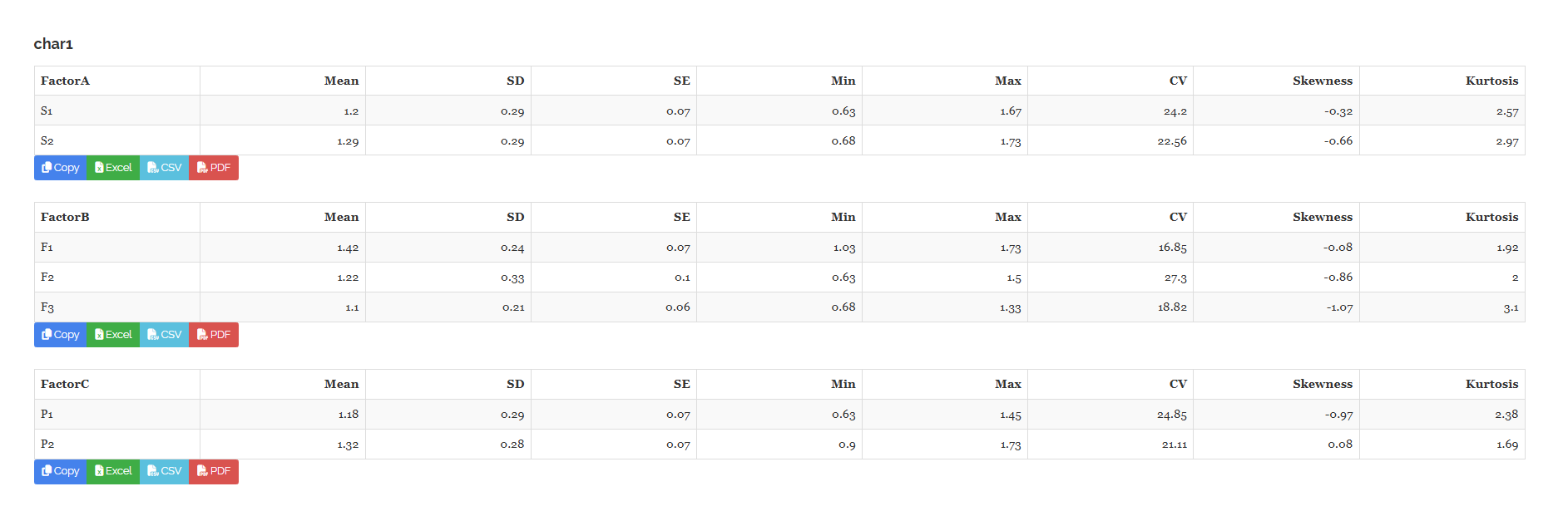
Between the main results and the plots, you will find two sub-tabs. The Summary stats tab (Figure 12) provides detailed information for each character. It does this separately for Factor A, Factor B, and Factor C. For each character, you will see the level Mean, SD (standard deviation), SE (standard error), Min (minimum), Max (maximum), CV (coefficient of variation), Skewness, and Kurtosis. These statistics help you understand the data before you move on to more complex analyses. Skewness and kurtosis are particularly important because they show you if a trait needs transformation, as described in Section 8. For example, with char1, six out of seven level blocks show mild negative skewness, ranging from \(-0.08\) for F1 to \(-1.07\) for F3. The exception is P2, which has a positive skewness value of \(+0.08\). The kurtosis values are all between \(1.69\) and \(3.10\). These values are typical and do not require any transformation. You can copy or export each block of data as an Excel, CSV, or PDF file.
The Individual ANOVA tab (Figure 13) allows you to analyse one trait at a time. First, select a trait from Select Character. The tab then displays the ANOVA table for that trait. This table includes columns for DF (degrees of freedom), MS (mean squares), F (F-value), and p.value (p-value). These columns are detailed for the block term, all seven treatment sources, and the error. For example, for char1, the table reports values for Block \(F = 22.24\) (\(p = 0.00\)), Factor A \(F = 2.24\) (\(p = 0.15\)), Factor B \(F = 10.20\) (\(p = 0.00\)), and Factor C \(F = 6.00\) (\(p = 0.02\)). It also includes four interactions with F-values ranging from \(0.10\) to \(0.25\) and p-values from \(0.63\) to \(0.91\). While Table 1 summarises each trait into a single column of mean squares, this tab provides a detailed classical ANOVA layout. This format is often required by journals in a methods appendix. After the ANOVA table, you will find the critical differences at 1% and 5%, the coefficient of variation (CV%), mean square error (MSE), standard error of the mean (SE(m)), and standard error of the difference (SE(d)) for each factor and interaction. Finally, it shows the level means with their groupings.

When you look at the table for char1, you will see that the Block row has the largest F value, which is \(22.24\) at \(p = 0.00\). This high F value indicates that the three blocks in your experiment are genuinely different from each other. It shows that including these blocks in your analysis was important. However, this does not mean that block R2 is the best treatment. Instead, it confirms that using a Randomized Block Design (RBD) was the right decision for your study. You should report this as evidence supporting the use of RBD, not as a conclusion about the treatments or factors themselves.
11 Visualising the results
When you look at numbers in a table, they can be convincing, but a picture can be even more persuasive. In RAISINS, you will find graphics organised into two sections: Basic Plots and Advanced Plots. In each section, you will see a row of icon buttons. To create a plot, click on the icon that represents the plot you want. After you click, a Plot Settings panel will appear next to the plot. Use this panel to select the factor for the x-axis and the response you want to plot. You can also choose the font style and decide on the export format for your plot. The available formats are PNG, JPEG, TIFF, PDF, and SVG.
11.1 Basic Plots
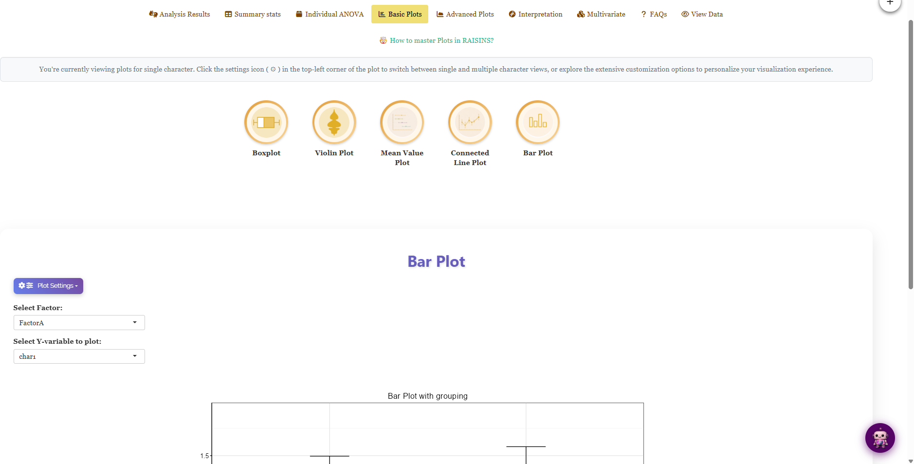
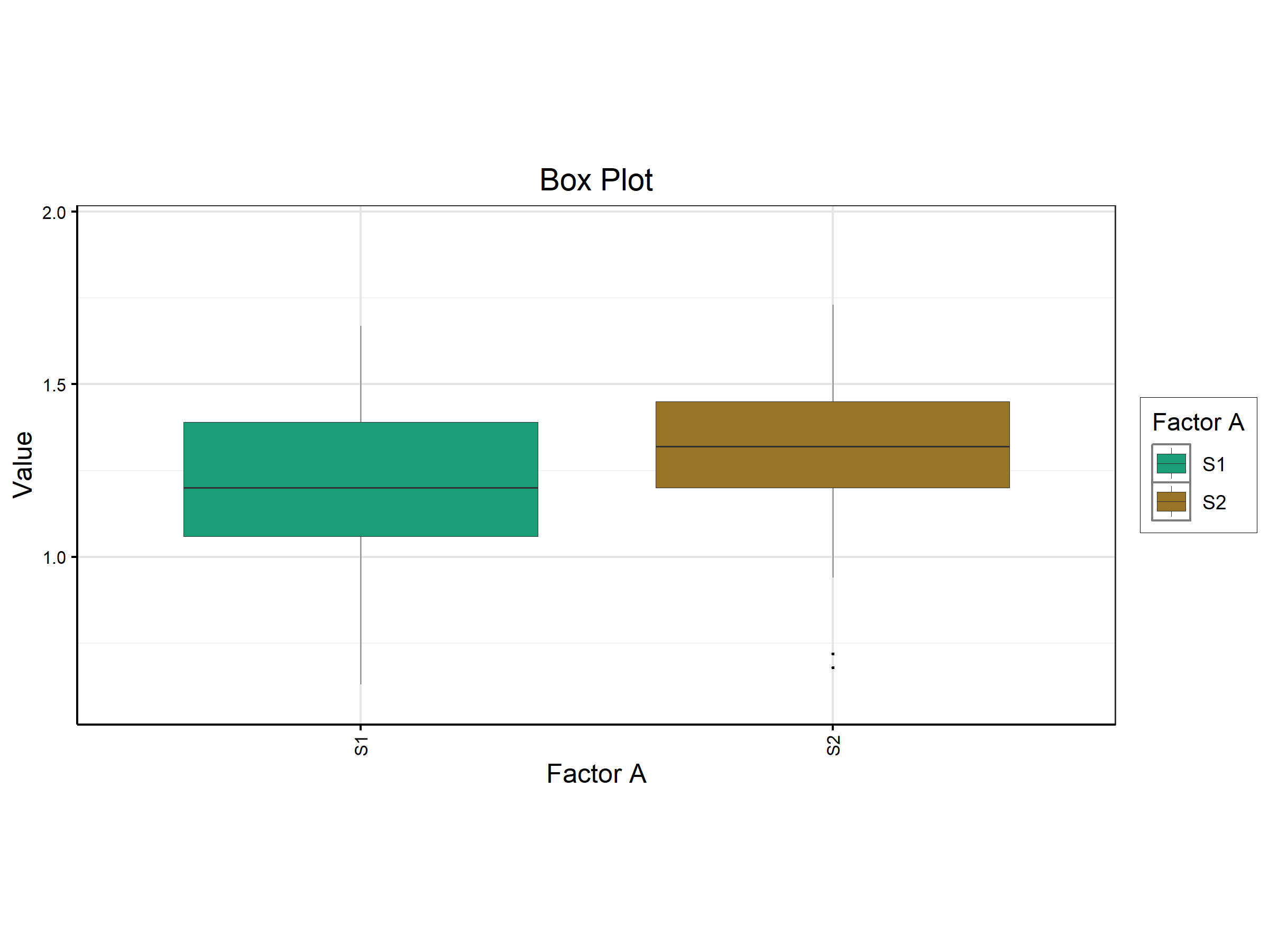
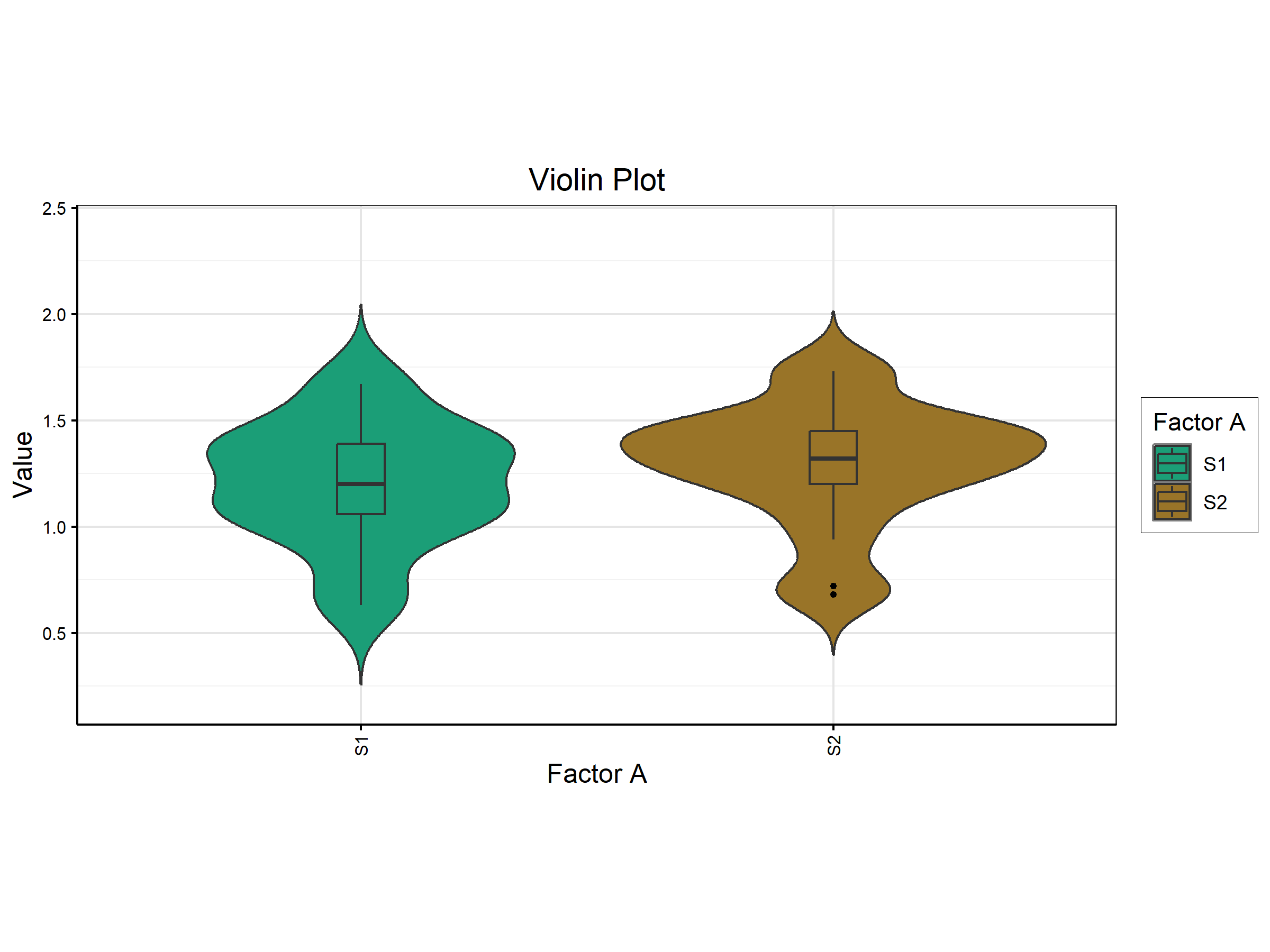
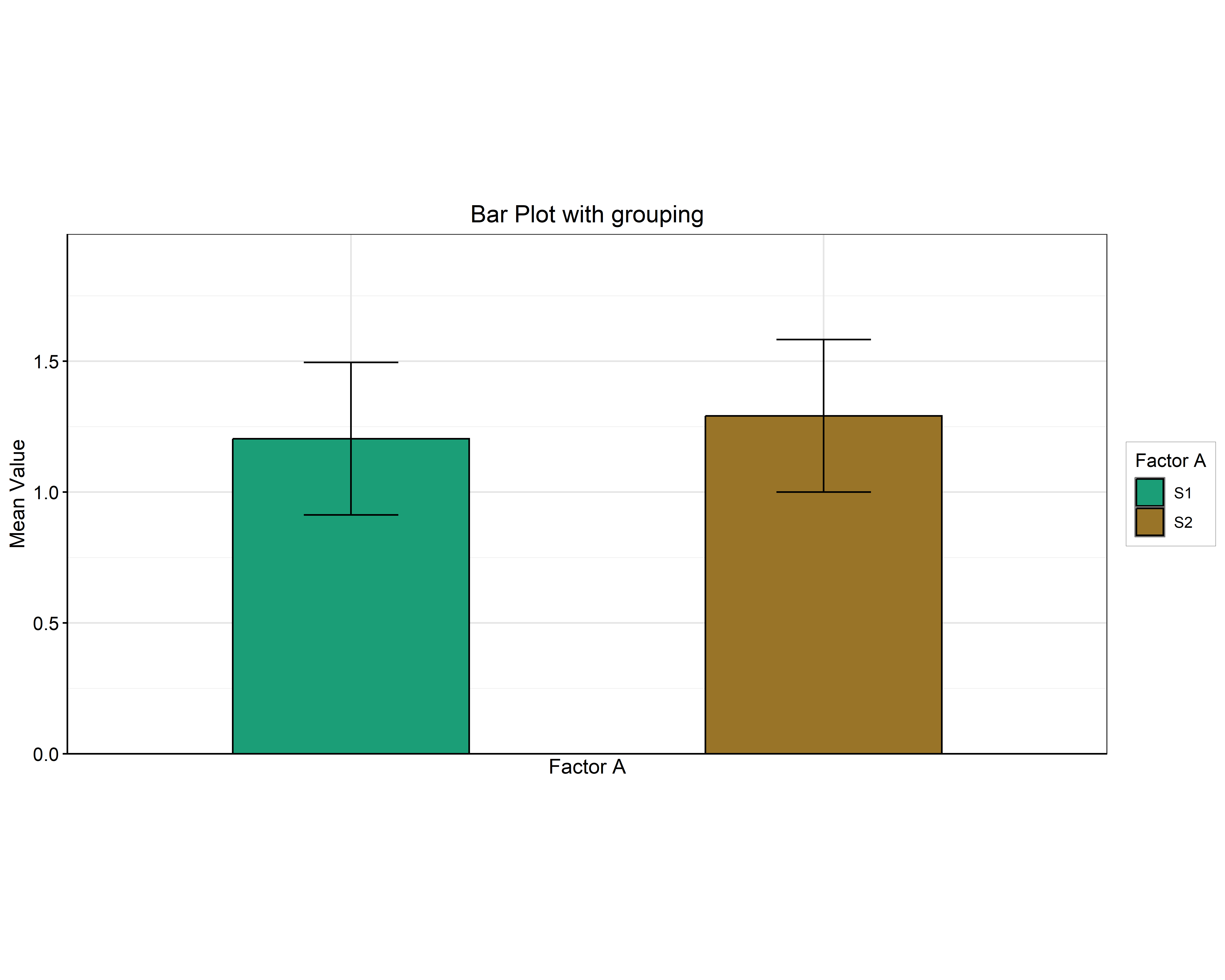
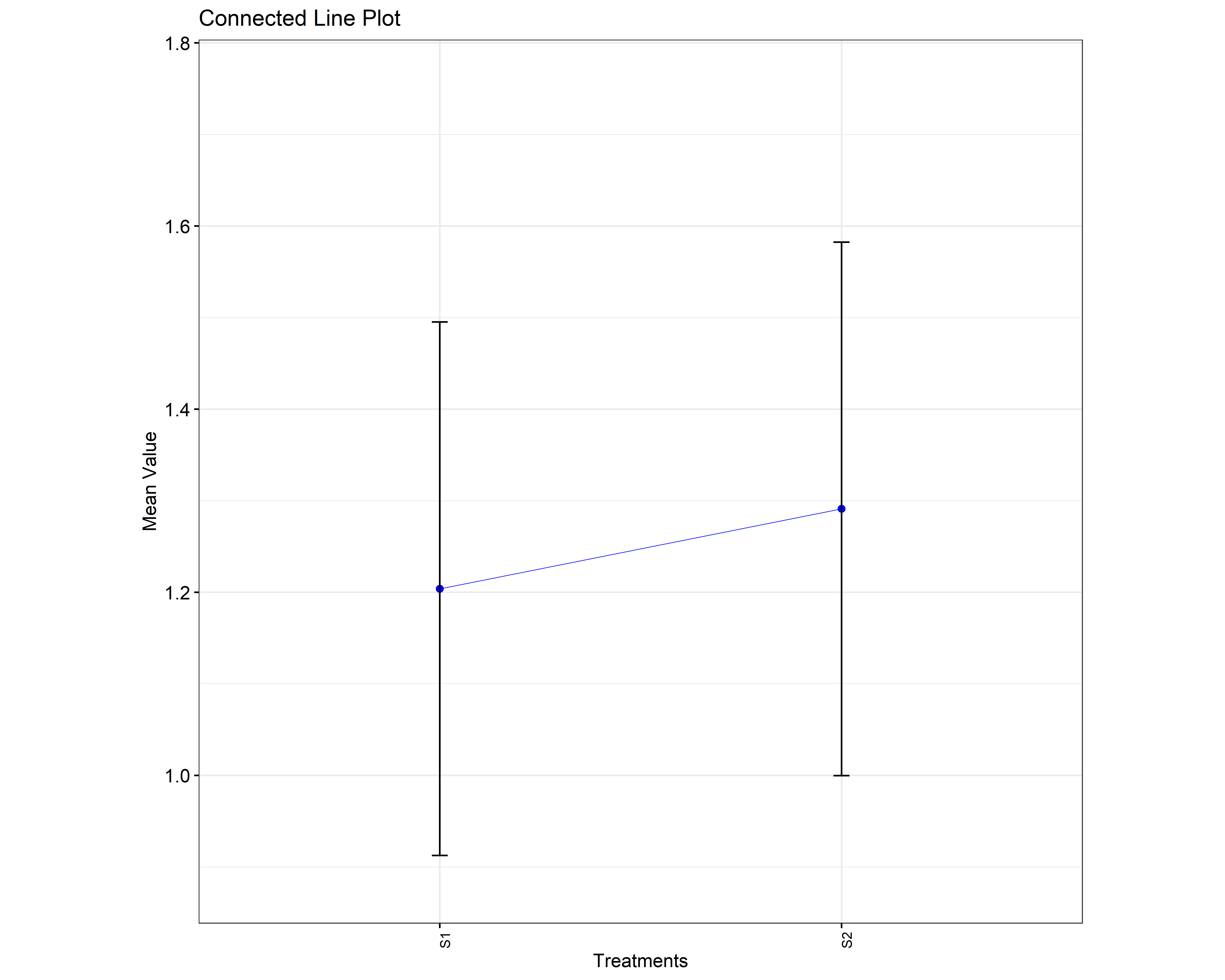
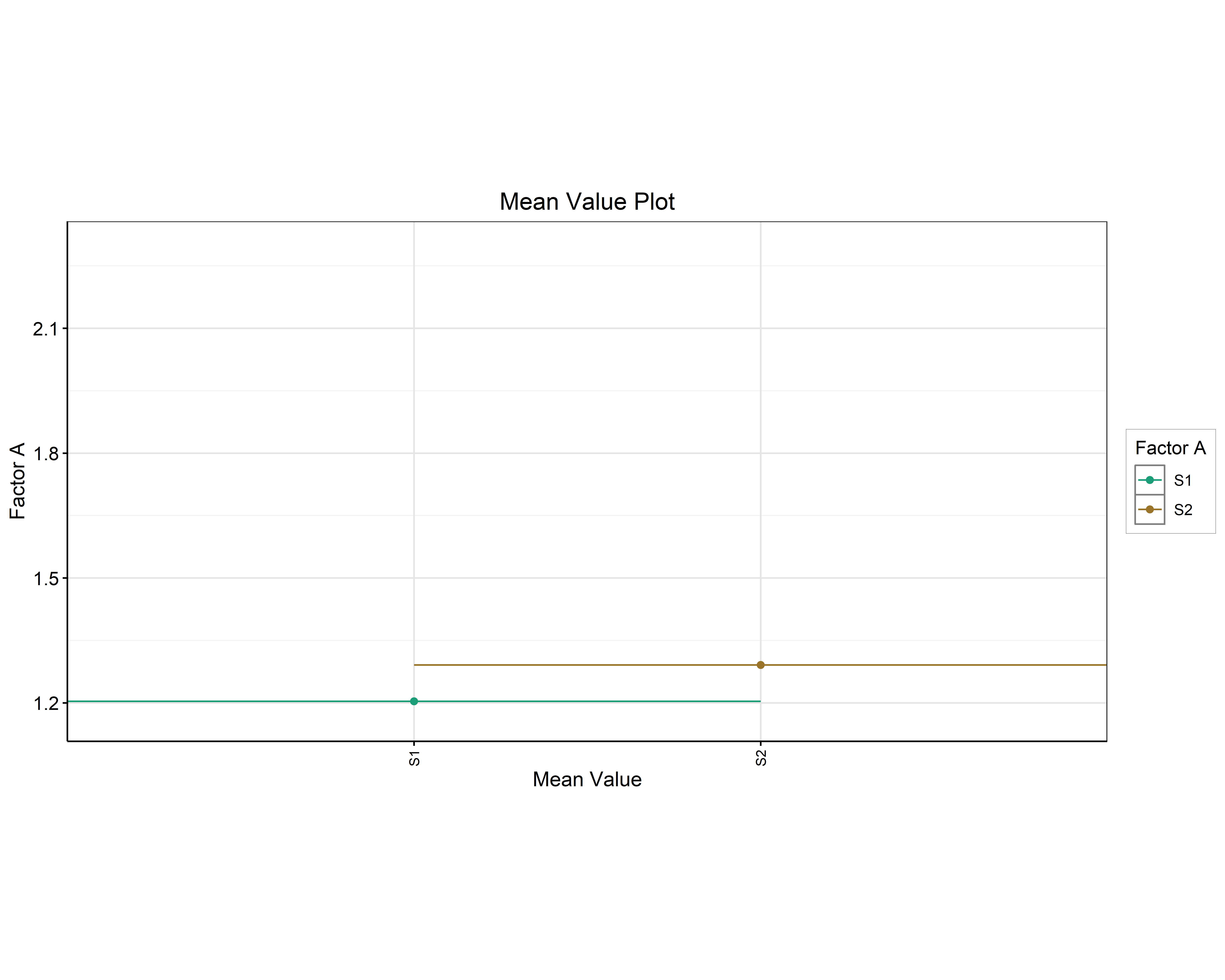
In the Basic Plots tab (Figure 14), you can create five common types of graphs: a Boxplot, a Violin Plot, a Mean Value Plot, a Connected Line Plot, and a Bar Plot. To begin, select a factor such as FactorA, FactorB, or FactorC using the Select Factor option. Then, choose the Y-variable you want to plot. This will display the chosen response variable across the different levels of the selected factor. At the top of the tab, a banner reminds you that you are currently viewing a single character. You can switch between single- and multiple-character views using the settings icon. Figure 15 illustrates the same comparison, showing char1 across the two levels of Factor A, using all five types of plots.
11.2 Advanced Plots
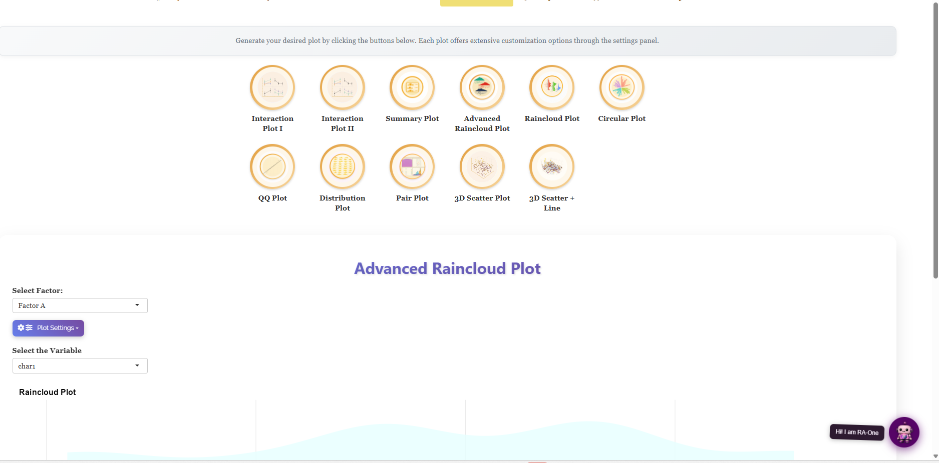
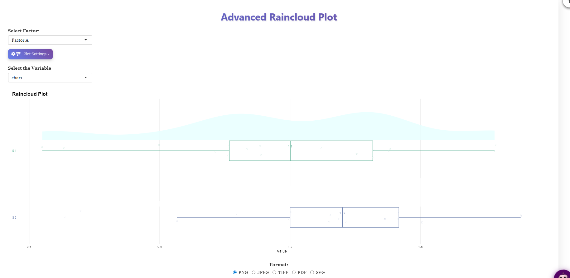
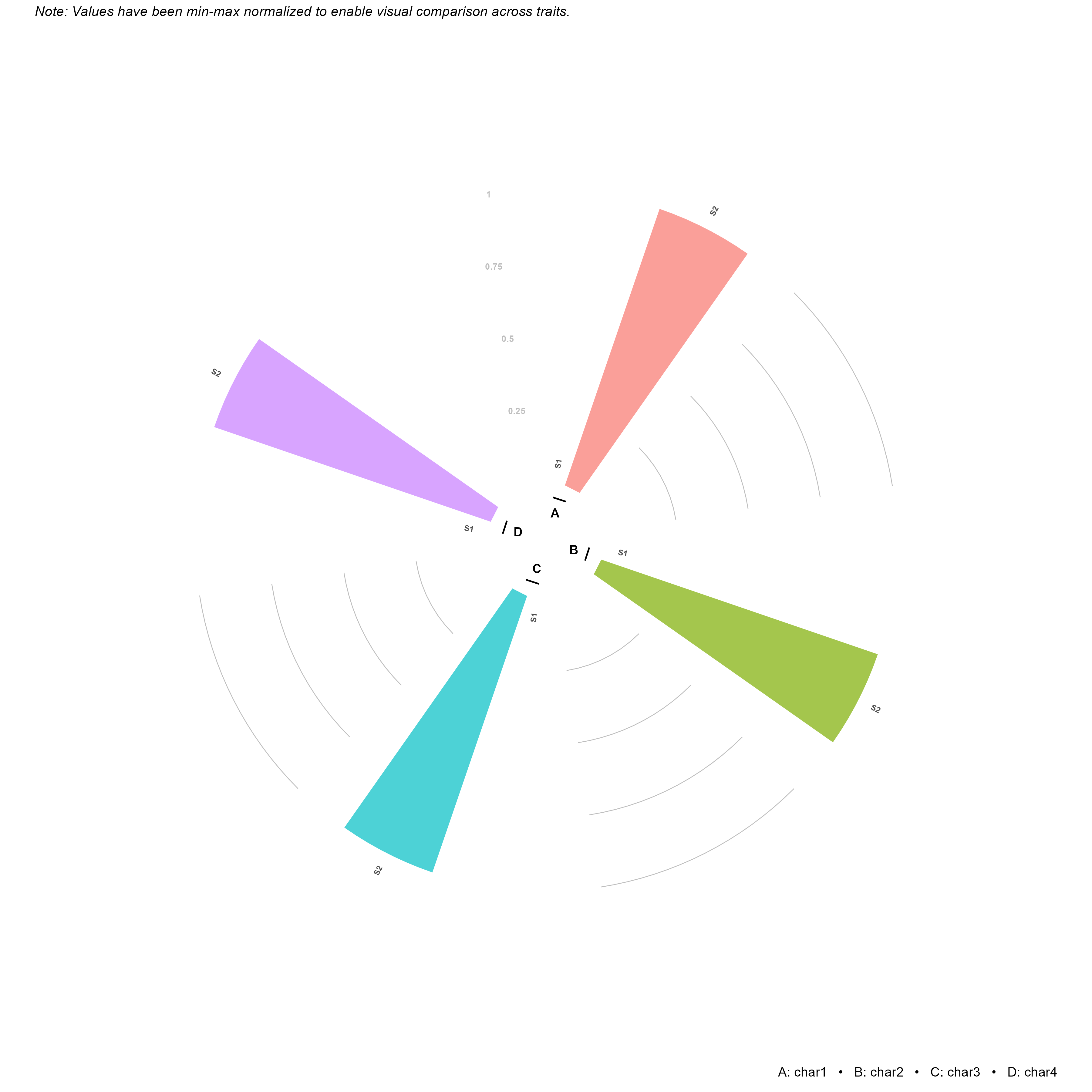
When you open the Advanced Plots tab (Figure 16), you find several specialised graphics options. These include Interaction Plot I and Interaction Plot II, which help you see how different factors interact with each other. The Summary Plot gives you an overview of your data. The Advanced Raincloud Plot and Raincloud Plot show data distribution and density in a visually appealing way. The Circular Plot is useful for displaying data in a circular format, often used for cyclical data. The QQ Plot helps you check if your data follows a particular distribution. The Distribution Plot shows how your data is spread out. The Pair Plot allows you to see relationships between pairs of variables. Lastly, the 3D Scatter Plot and 3D Scatter + Line views let you explore data in three dimensions. For each of these plots, you have controls to Select Factor and Select the Variable you want to analyse. You can also adjust settings in the Plot Settings panel to customise your plots.
The interaction plot
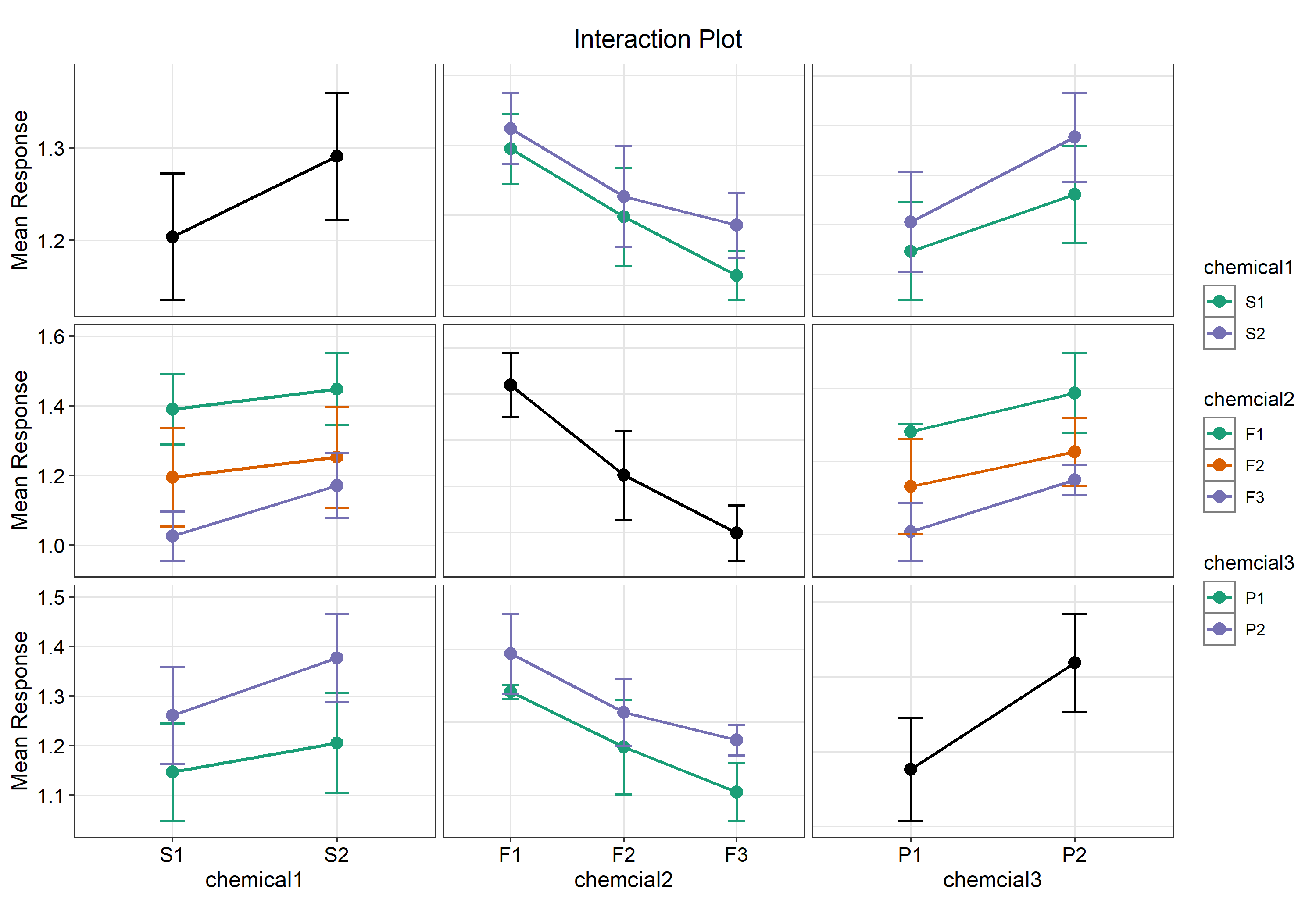
The Interaction Plot is crucial because it visually represents the main question your experiment is designed to answer. In a three-factor experiment, this plot appears as a 3 × 3 grid of panels (Figure 17). Understanding the layout will help you read it more easily. Each column in the grid has an x-axis labelled with a factor name: chemical1, chemical2, and chemical3, from left to right. The three panels on the diagonal are in black and do not have a legend. These panels show the main effect of each factor, which is the average response at each level of that factor, along with error bars. The six off-diagonal panels display the two-way interaction profiles. In these panels, the average response is plotted against the column factor, with different coloured lines representing each level of a second factor. Since each pair of factors is shown twice, once in each orientation, you can choose the view that makes the interaction easier to understand.
Reading the grid is then a matter of looking at the slopes:
- Parallel lines mean the vertical gap between them is the same at every level of the x-axis factor, so one factor’s effect does not depend on the other. There is no interaction.
- Lines that fan apart, converge, or cross mean the gap changes, so the effect of the x-axis factor differs between the coloured levels. That is an interaction, and a crossing is its strongest form, the ranking of the levels actually reverses.
- The black diagonal panels should be read last. When an off-diagonal panel shows crossing lines, the corresponding main-effect panel is an average over lines that disagree with one another, and quoting it alone would be misleading.
Figure 17 generates a visual representation called char1. According to Figure 11, this chart shows significant effects from Factor B and Factor C, but no significant interaction between them. The grid on the screen illustrates this clearly. There are three black diagonal panels that display the main effects. In the first panel, chemical1 shows a gentle increase from S1 to S2, indicating a non-significant effect as seen in Table 2. In the second panel, chemical2 decreases steadily from F1 through F2 to F3, highlighting a strong effect as shown in Table 3. In the third panel, chemical3 increases from P1 to P2, reflecting the effect in Table 4. The six coloured panels show lines that run almost parallel, never crossing and maintaining a consistent distance apart. For example, in the middle-left panel, the lines for F1, F2, and F3 rise together from S1 to S2 without changing their order. Similarly, in the bottom-middle panel, the lines for P1 and P2 descend together from F1 to F3, keeping roughly the same distance between them. This visual parallelism corresponds to the four NS interaction rows in the ANOVA table, indicating no significant interaction.
When you change Select the Variable to char3, the grid changes significantly. You will see the F3 line crossing the other lines. This crossing pattern is a visual representation of an \(F = 156.12^{**}\) B × C interaction.
When you have a significant interaction in your data, it is helpful to show both an interaction plot and an interaction table together. The plot visually shows how the effect of one factor changes depending on another factor. For example, if you have two treatments and their effects differ based on the time of day, the plot will make this clear immediately. The interaction table, on the other hand, provides detailed information with its CD (Critical Difference) values and letter groupings, which confirm the significance of these changes. This combination is particularly useful in a three-factor design, where you have twelve cell means. These means can be difficult to understand just by looking at numbers, so the plot and table together make the information clearer and easier to interpret.
The remaining advanced graphics help you understand more than just one comparison. They show you the shape of the data and how different traits relate to each other. Figure 18 brings together four of these graphics.
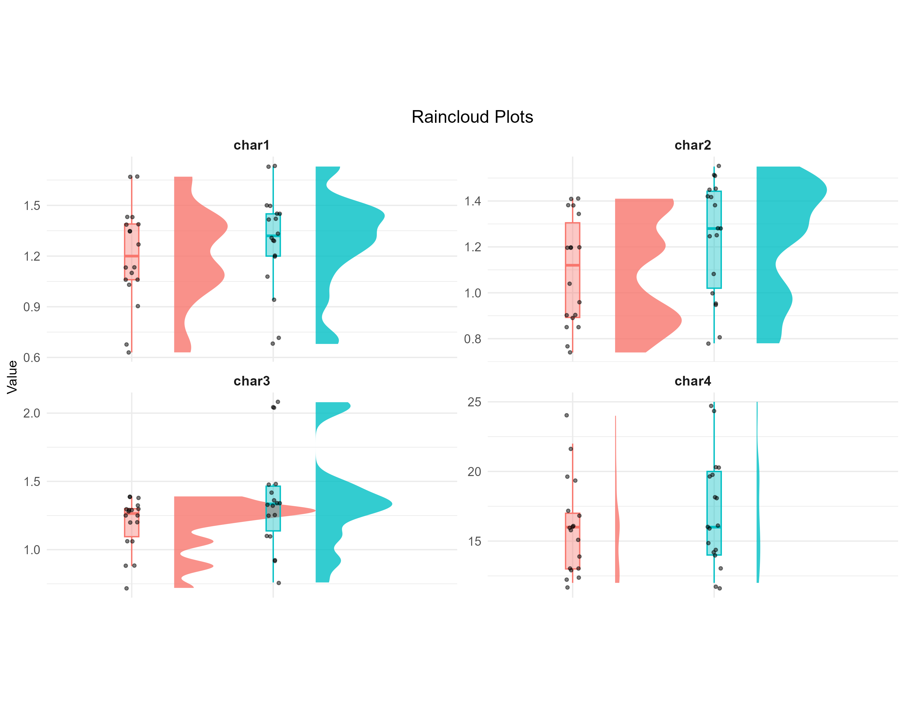
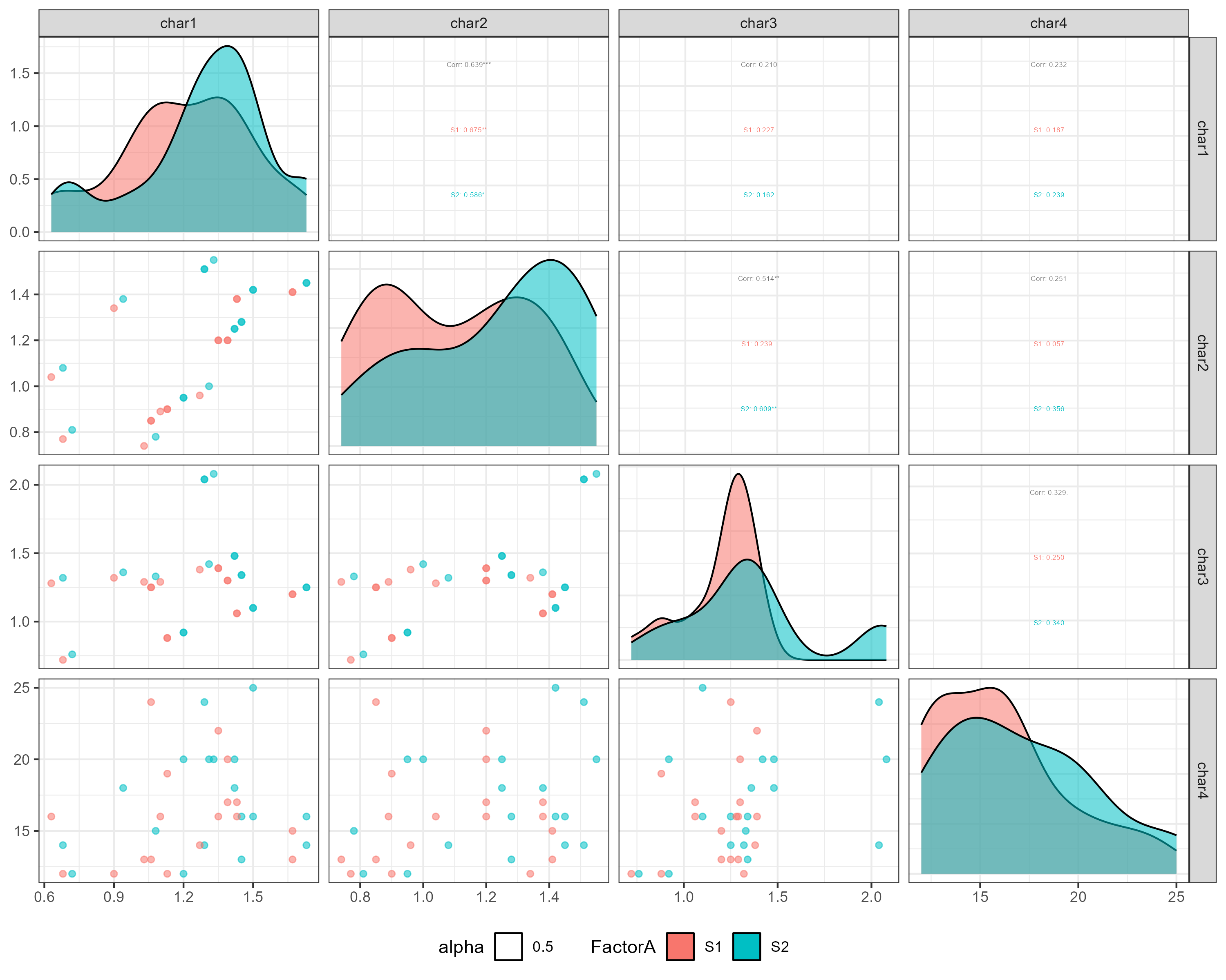
The pair plot shows how each pair of traits is related to each other. For example, the correlation between char1 and char2 is \(0.639\), which is significant at the 0.1% level. This means there is a strong relationship between these two traits. Similarly, the correlation between char2 and char3 is \(0.514\), significant at the 1% level, indicating a notable relationship. However, the correlations between char1 and char3 (\(0.210\)), char1 and char4 (\(0.232\)), char2 and char4 (\(0.251\)), and char3 and char4 (\(0.329\)) are weaker and not significant. These correlations are important because they help explain the PCA index of Section 12. The PCA index summarises the data by condensing these relationships into a single component. This is why one component can account for a large portion of the variation in the data. Since char4 is the least correlated with the other traits, it contributes the least to this component.
12 Looking at all traits together: MANOVA and PCA index
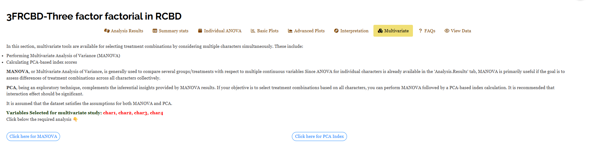
When you are analysing your data, the Analysis Results tab allows you to test each trait individually. This means you can see how each trait responds to different treatments one by one. However, there are times when you need to understand how treatments affect all traits together. You might also want to combine multiple traits into a single selection index for a more comprehensive analysis. This is where the Multivariate tab (Figure 19) becomes useful. It shows you the response variables that are part of the multivariate study. It also provides two options: one button labelled Click here for MANOVA and another labelled Click here for PCA Index. MANOVA, or Multivariate Analysis of Variance, helps you determine if there are any differences in the treatments when considering all traits together. The PCA Index, or Principal Component Analysis Index, allows you to combine the traits into a single index, simplifying the selection process.
12.1 MANOVA across all responses
In MANOVA (Multivariate Analysis of Variance), you check if different treatments have distinct effects when you consider multiple characteristics, like char1 to char4, as a single group. You fit a full three-factor model, including a block term, to see these effects. The output shows Pillai’s trace, a strong test statistic, which is converted into an F-value. This helps you understand if the treatments differ. Additionally, you get a partial \(\eta^2\) effect size for each source (Figure 20), which tells you the strength of each treatment’s effect.
In this dataset, every source of variation is significant. This includes the block term and all the factors. The significant sources are: Block (\(F = 2.66\), \(p = 0.02\), \(\eta^2 = 0.35\)), Factor A (\(F = 12.27\), \(p = 0.00\), \(\eta^2 = 0.72\)), Factor B (\(F = 6.18\), \(p = 0.00\), \(\eta^2 = 0.55\)), Factor C (\(F = 13.22\), \(p = 0.00\), \(\eta^2 = 0.74\)), the interaction between A and B (A × B, \(F = 2.79\), \(p = 0.01\), \(\eta^2 = 0.36\)), the interaction between A and C (A × C, \(F = 6.04\), \(p = 0.00\), \(\eta^2 = 0.56\)), the interaction between B and C (B × C, \(F = 6.79\), \(p = 0.00\), \(\eta^2 = 0.58\)), and the three-way interaction among A, B, and C (A × B × C, \(F = 3.48\), \(p = 0.00\), \(\eta^2 = 0.41\)). It is important to note that Factor A is significant in this multivariate analysis, even though it was not significant for individual traits char1 and char4. Similarly, the block term is significant here, even though blocks were only important for two out of the four traits. This means that when you look at all four traits together, the treatments and blocks show a pattern that you cannot see when looking at each trait separately. This is the purpose of a multivariate test: to reveal patterns across multiple variables that are not visible when examining them one by one.
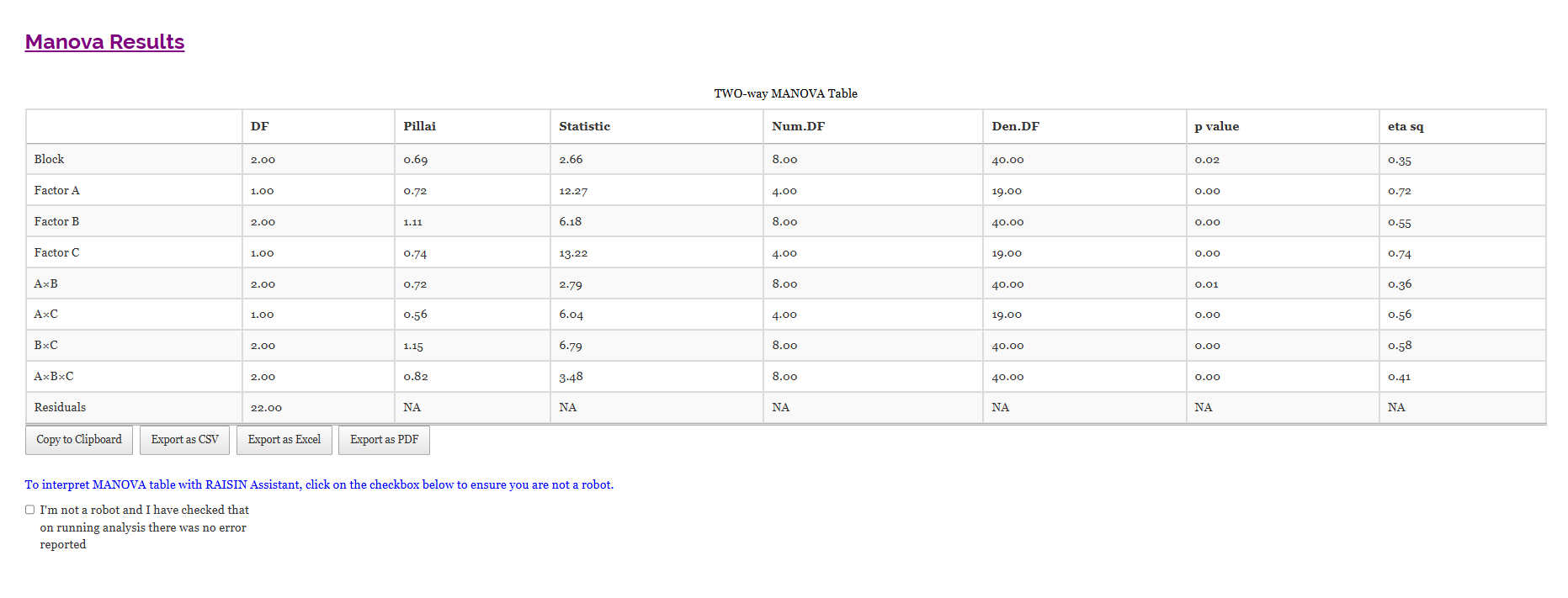
When you look at the table, you will see the heading TWO-way MANOVA Table. This heading is a fixed label and does not describe your specific model. To understand what was actually analysed, focus on the rows of the table. These rows show the components that were included in the analysis: Block, Factor A, Factor B, Factor C, and all the interactions between them, including A × B × C. Pay attention to these rows to know what was fitted in your model, rather than relying on the heading.
12.2 PCA-based index score
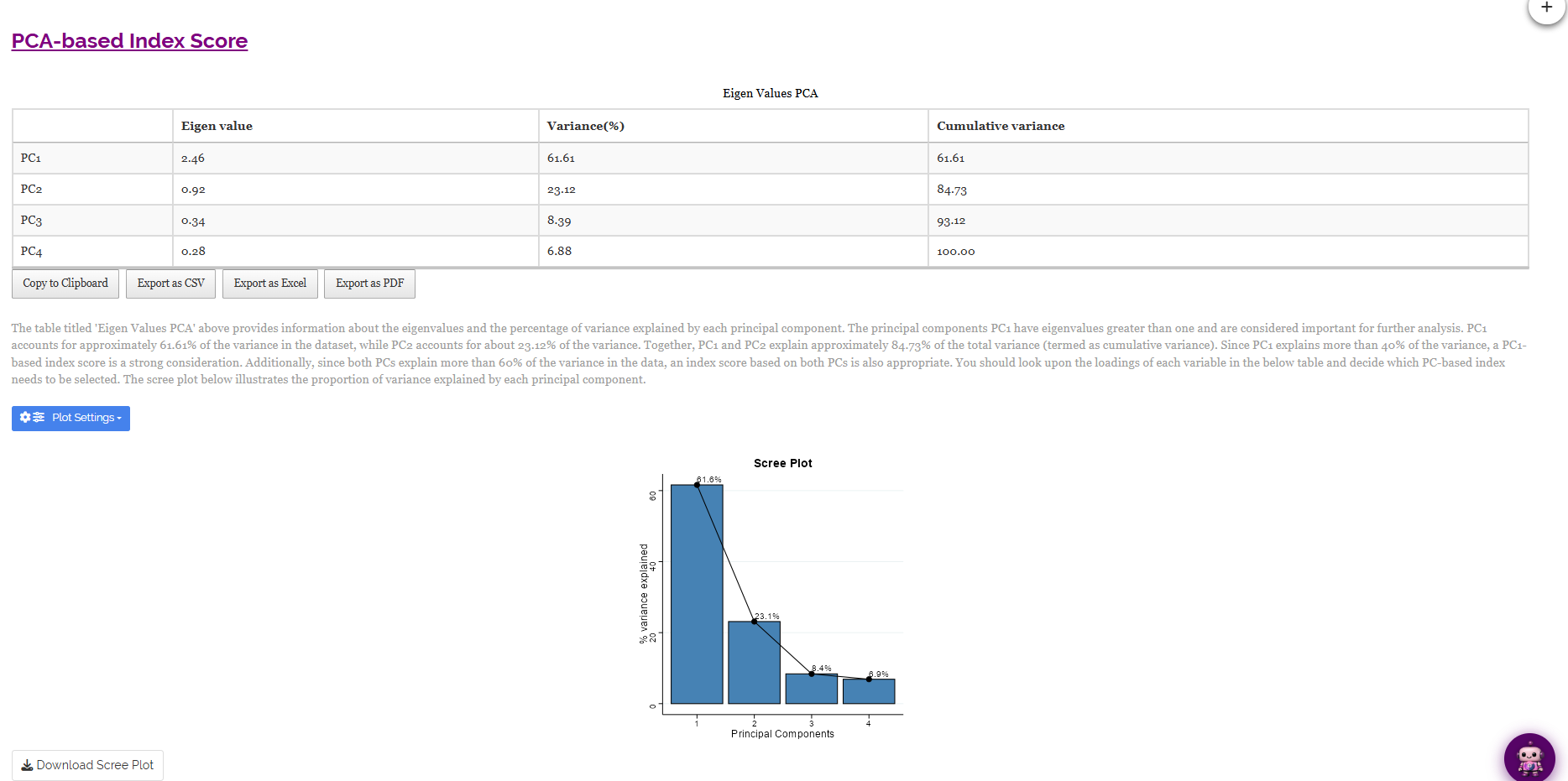
When you want to rank treatment combinations based on all traits at once, you can use a PCA-based index. PCA, or Principal Component Analysis, helps you by reducing the number of correlated traits into a few independent components. These components are then used to build a score. In this dataset (Figure 21), the first principal component, PC1, has an eigenvalue of 2.46 and explains 61.61% of the total variance. The second principal component, PC2, adds another 23.12%. Together, PC1 and PC2 account for 84.73% of the total variance. Since PC1 alone explains more than 40% of the variance, using a PC1-based index is a good choice. Additionally, since both components together explain more than 60%, using a two-component index is also reasonable. The scree plot below the table visually represents this information. It shows a sharp drop from 61.6% to 23.1% and then levels off, indicating the variance explained by each component.
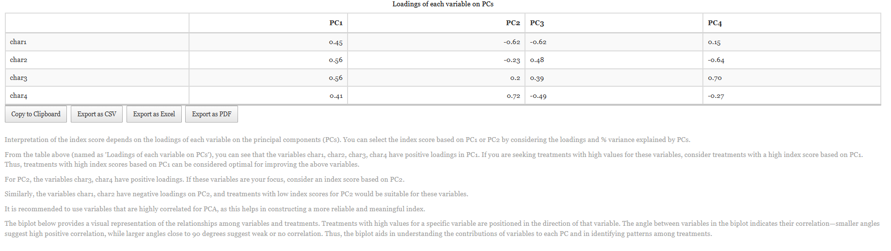
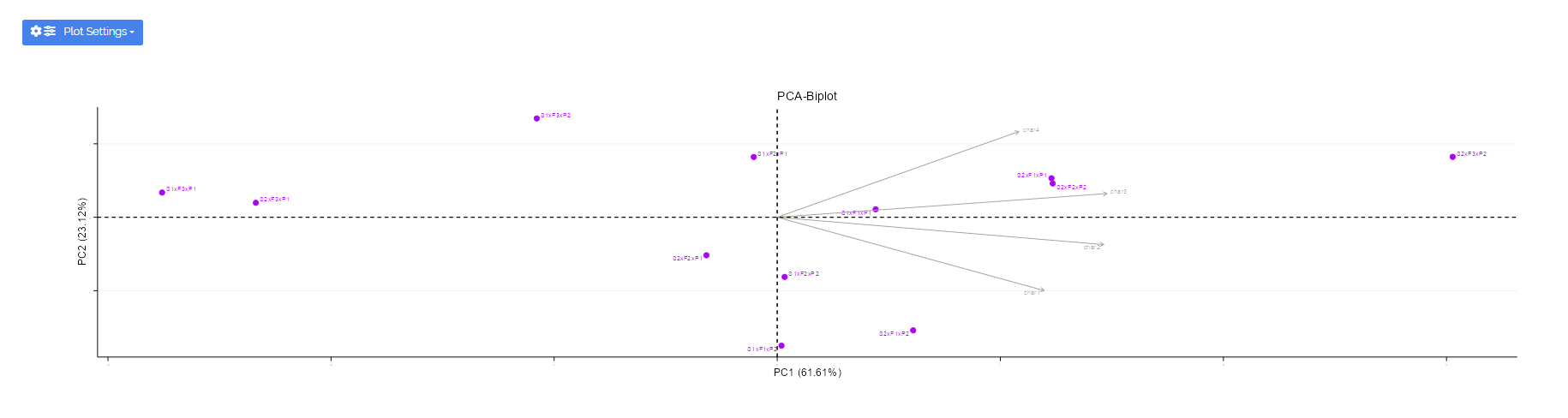
The loadings table (Figure 22) helps you understand which traits influence each component. This allows you to determine if the index measures what you intend. For PC1, all four traits have positive loadings. Char2 and char3 have the strongest influence at \(0.56\) each, followed by char1 at \(0.45\) and char4 at \(0.41\). A high score on PC1 indicates “high on everything,” making it a useful general index in this context. In contrast, PC2 separates the traits rather than combining them. Char4 (\(0.72\)) and char3 (\(0.20\)) have positive loadings, while char1 (\(-0.62\)) and char2 (\(-0.23\)) have negative loadings. This means a PC2 index would rank treatments that favour char4 over char1. The biplot (Figure 23) visually represents this information. It shows the four trait arrows spreading to the right, with the twelve treatment combinations positioned along these arrows.
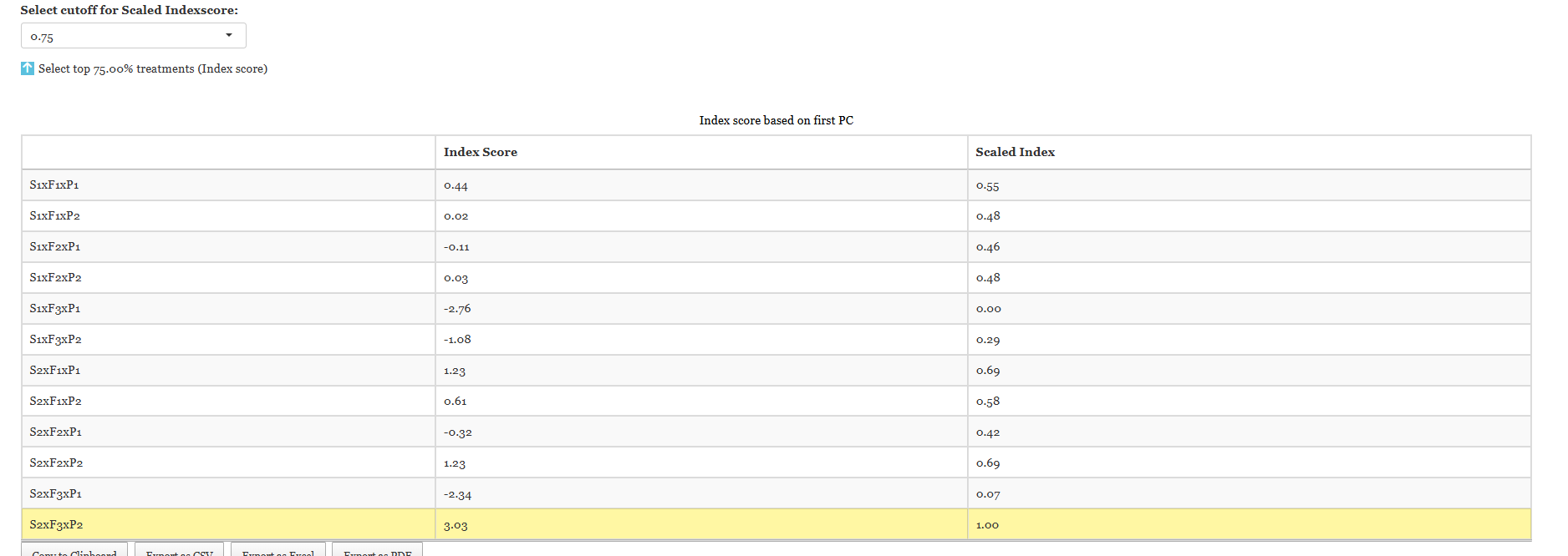
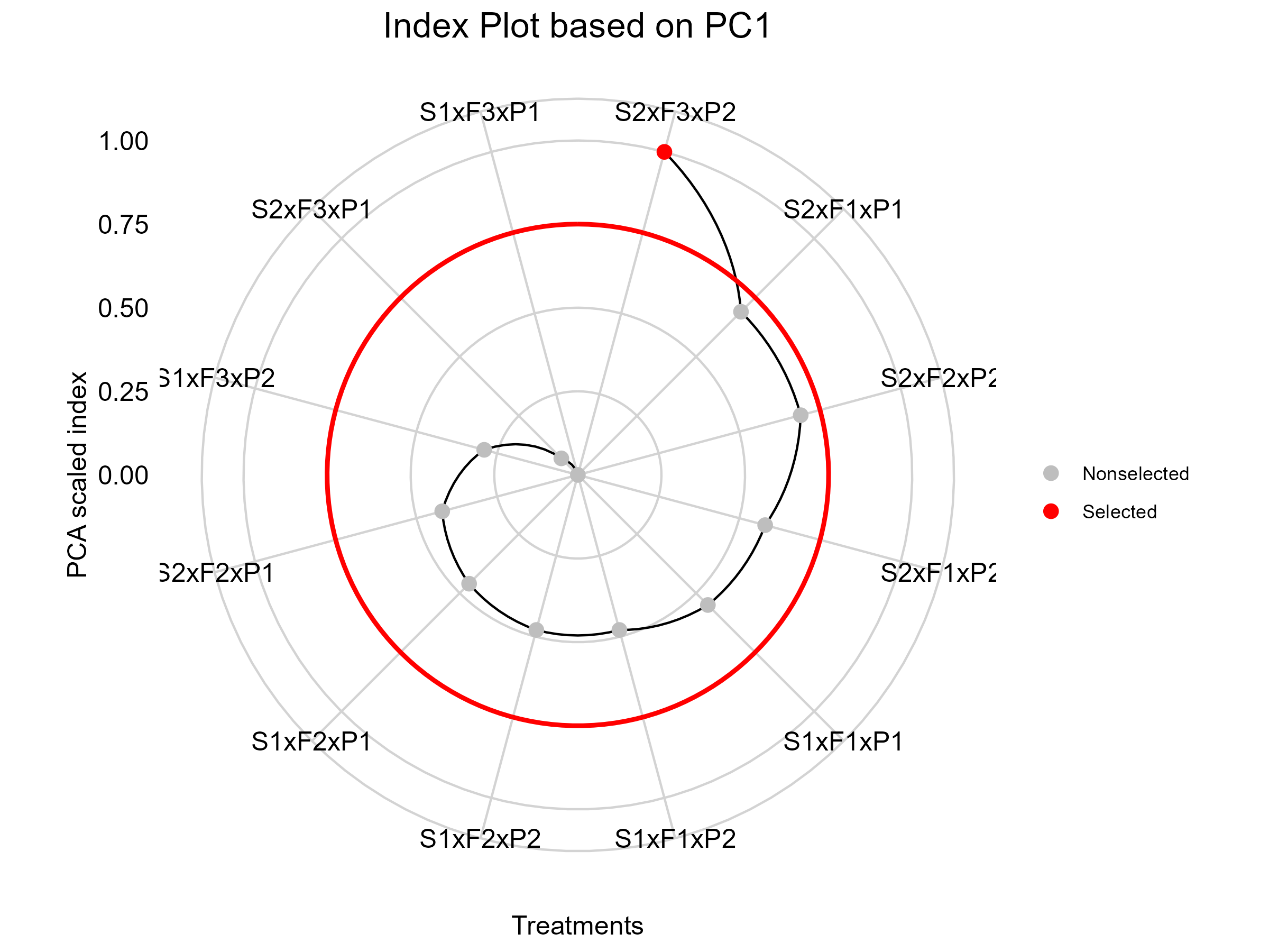
First, you choose an index to evaluate the treatment combinations. The application converts this index into a scaled score ranging from 0 to 1 (Figure 24). You then use the Select cutoff for Scaled Index Score control to highlight the top percentage of treatment combinations based on this score. For example, if you set the cutoff at 0.75, only one combination qualifies: S2×F3×P2. This combination has a raw index score of \(3.03\) and a scaled index of \(1.00\), which is more than twice as high as the next-best score. Following this top combination are S2×F1×P1 and S2×F2×P2, both with a raw score of \(1.23\) and a scaled score of \(0.69\). At the lower end, you have S1×F3×P1 with a raw score of \(-2.76\) and a scaled score of \(0.00\), and S2×F3×P1 with a raw score of \(-2.34\) and a scaled score of \(0.07\). The Index Plot (Figure 25) visually represents these rankings on a dial. The selected combination appears in red outside the cutoff circle, while the eleven non-selected combinations are shown in grey inside the circle.
You have reached a point where both the multivariate analysis and the univariate tables show the same results. In Table 8, the combination S2×F3×P2 has the highest values for both char2 and char3. Similarly, S1×F3×P1 has the lowest values for both. The index, which is calculated using a different method, also identifies these same two combinations as the highest and lowest. This agreement confirms the consistency of your findings across different analytical methods.
When you use MANOVA (Multivariate Analysis of Variance), you are trying to find out if any treatment has a different effect on a group of traits when considered together. This is called an inferential approach because you are making inferences about the treatments based on the data. On the other hand, PCA (Principal Component Analysis) is used to explore how you can combine these traits into a single index. This index helps you rank the treatments. PCA is exploratory because it helps you discover patterns in the data without making specific predictions. These two methods work well together. However, you should be careful when using the PCA index if the interaction between factors is not significant. This is because ranking a single “best combination” of traits is less clear when interactions are not significant. In this case, the three-way interaction is significant in both the univariate ANOVA and the MANOVA. This means that ranking treatments based on a combination of traits is meaningful and reliable.
13 Interpretation
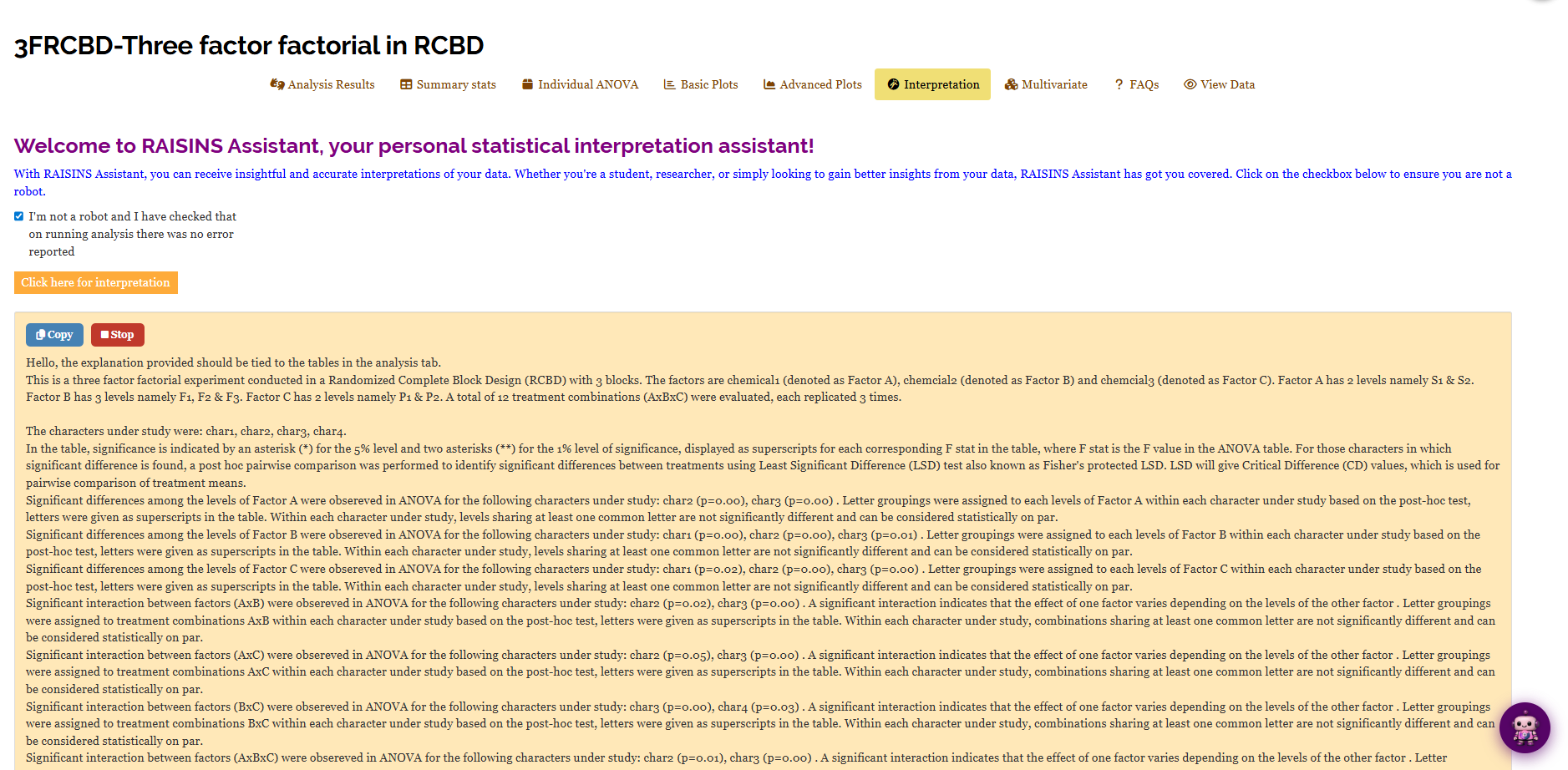
RAISINS provides a plain-language interpretation of your results so you can understand the findings without decoding the tables yourself. Open the Interpretation sub-tab, tick the box confirming that the analysis ran without error, and click Click here for interpretation (Figure 26). RAISINS restates the design, three factors in a Randomized Complete Block Design with 3 blocks, Factor A at levels S1 and S2, Factor B at F1, F2 and F3, Factor C at P1 and P2, twelve treatment combinations replicated three times, and then reads every source in turn.
This dataset shows significant differences for various factors and their interactions across different characteristics. For Factor A, there are significant differences in char2 (\(p = 0.00\)) and char3 (\(p = 0.00\)). Factor B shows significant differences in char1 (\(p = 0.00\)), char2 (\(p = 0.00\)), and char3 (\(p = 0.01\)). Factor C has significant differences in char1 (\(p = 0.02\)), char2 (\(p = 0.00\)), and char3 (\(p = 0.00\)). The interaction between Factors A and B is significant for char2 (\(p = 0.02\)) and char3 (\(p = 0.00\)). For the interaction between Factors A and C, significant differences appear in char2 (\(p = 0.05\)) and char3 (\(p = 0.00\)). The interaction between Factors B and C shows significance in char3 (\(p = 0.00\)) and char4 (\(p = 0.03\)). Lastly, the three-way interaction A × B × C is significant for char2 (\(p = 0.01\)) and char3 (\(p = 0.00\)). These findings align with the flags in Figure 11. Additionally, for each source, the dataset explains the letter groupings and identifies which levels are statistically equivalent. This information is formatted to be easily included in a results section.
When you interpret the results, remember that the interpretation comes from the same calculations as the tables. Use it as a guide alongside the tables, not as a replacement. Keep Figure 11 open next to the interpretation. Make sure the p-values mentioned in the text match the flags in the table exactly. This is the fastest way to verify that you have chosen the correct columns. Pay special attention to ensure that you have directed Select the blocks to the block column and not mistakenly to a response column.
14 Chat with your data using RA-One
RA-One is a conversational assistant designed for the three-factor factorial RBD module. You can find it under the RA-One tab. You interact with it by asking questions in plain language. It responds using the results from your specific analysis, not general statistical advice. This means every result it talks about comes directly from what the module has calculated. It never makes up numbers. If a value is not available, it will inform you rather than guess. All its answers are in plain English, without any code or software commands.
When your results are ready, the screen presents you with several options to help you understand them. You can choose Guide me through my results if you want a step-by-step explanation of what your data shows. If you select Interpret results, you will get a summary of how significant each character is in your study. The Best treatment option helps you identify which combination of treatments performs best across all the variables you are examining. If you need assistance in drafting your report, choose Report results. Additionally, you have the option to type in your own questions. For example, you might ask, “Is the three-way interaction significant for any trait?” or “Which level of chemical2 gives the highest char1?” These features are designed to make it easier for you to analyse and interpret your data effectively.
Figure 27 provides the answer to Interpret my results. RA-One begins by summarising the experiment: it involves two levels of Factor A (chemical1), three levels of Factor B (chemical2), two levels of Factor C (chemical3), four response variables, and three blocks. A block is a complete replication of every treatment combination, grouped to control unwanted variation. The analysis then examines each character individually. For char1, it finds Factor B significant (\(p = 0.0000\)) and Factor C significant (\(p = 0.0200\)), with all four interactions being non-significant. For char2, it identifies all three factors as significant, along with the interactions A × B (\(p = 0.0200\)), A × C (\(p = 0.0500\)), and the three-way interaction A × B × C (\(p = 0.0100\)). For char3, it reports that all three factors and all four interactions are significant at \(p = 0.0000\). This is the same information provided by the Interpretation tab, but presented in a conversational manner, addressing one question at a time.
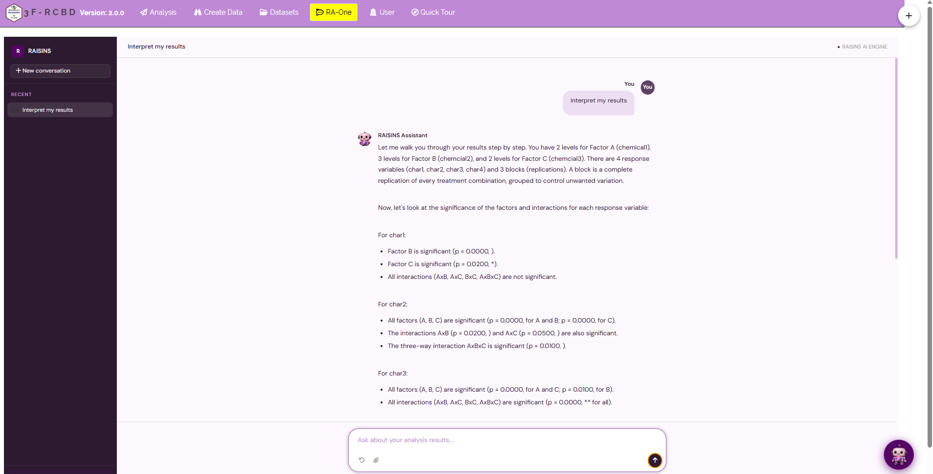
In one conversation, you can use RA-One to understand your results. It helps you create a data template (Section 7.4) and retrieves the model dataset (Section 7.3). It also guides you through the tables. This means you can conduct most of a routine three-factor factorial Randomized Block Design (RBD) session without leaving the chat window.
15 FAQs
The module has a FAQs sub-tab that provides detailed answers and practical tips about the features mentioned earlier. Here are some common questions you might find helpful: “What is Cohen’s F in the results?” This question helps you understand the effect size measure used in your analysis. “How is the transformation algorithm applied?” This explains the process used to transform your data for better analysis. “What does a significant Block row mean?” This tells you about the importance of blocking in your experimental design. “Why should I read the three-way interaction before the main effects?” This guides you on the order of interpreting interactions and main effects in your results. Another question, related to the control described in Section 8, is “When should I use P-adjustment?” This explains that the P-adjustment option is relevant for LSD tests and advises when to choose methods like Bonferroni, Holm, or Benjamini–Hochberg. It also clarifies why the CD and p-value rows disappear once an adjustment is activated.
16 View data
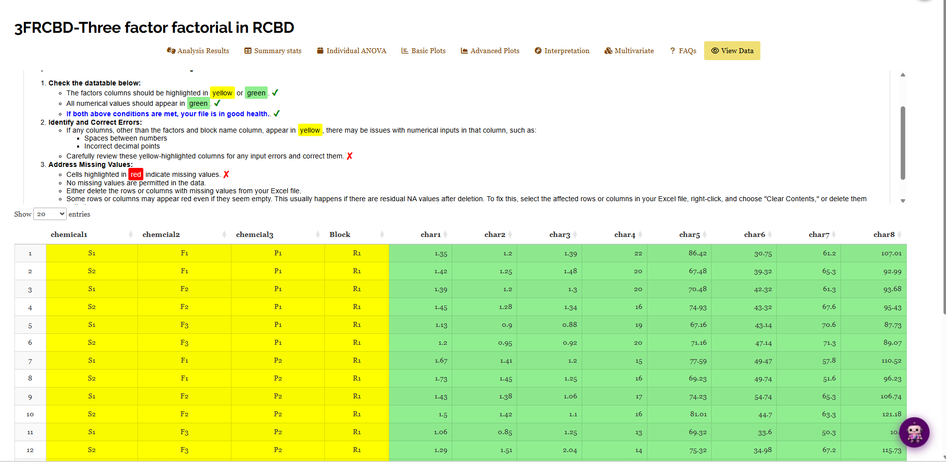
When you upload your dataset, you should first use the View Data tool. This is your main way to check that your data is correct before you start analysing it (Figure 28). As soon as you upload the dataset, the system automatically performs a Health Check. This check highlights any issues by colouring the table, making it easy for you to spot problems right away.
- The factor and block columns should be highlighted in yellow or green, and all numerical values in green. If both conditions are met, your file is in good health.
- If a column that should be numeric appears in yellow, there is something wrong with its contents, typically spaces between numbers or an incorrect decimal point. Review that column in your spreadsheet and correct it.
- Cells highlighted in red indicate missing values, which are not permitted. Delete the affected rows or columns in your Excel file. A row or column that looks empty but still shows red usually carries residual
NAvalues; select it, right-click, and choose Clear Contents, or delete it outright.
In Figure 28, you will see that the four label columns-chemical1, chemical2, chemical3, and Block-are highlighted in yellow. This indicates they are in a healthy state. Additionally, every character column is shown in green, which is also a sign of a healthy state. When working with a three-factor Randomized Block Design (RBD), you can use this table to visually confirm the design. To do this, set Show entries to 20. Then, check that rows 1 to 12 belong to block R1 and that they include all twelve treatment combinations exactly once before block R2 starts. If you notice any issues flagged in this table, address them before relying on the results.
17 Wrapping up
In a three-factor factorial Randomized Block Design (RBD), you want to find out if three factors work independently or if the effect of each factor depends on the others. To do this, you use several tools and analyses. First, you look at the ANOVA summary, which includes a block row and seven treatment rows. This helps you see how the treatments perform. Next, you examine three separate tables, each focusing on one of the factors. Then, you check three two-way interaction tables to see how pairs of factors interact. After that, you review a three-way table to understand how all three factors might interact together. An interaction plot visually shows these interactions. You also use MANOVA (Multivariate Analysis of Variance) and PCA (Principal Component Analysis) index to get a deeper understanding of the data. Finally, a written interpretation helps you make sense of all these analyses. If the analyses show that the factors interact, they guide you on which treatment combination to choose.
Let’s break this down step by step. Imagine you are looking at a table of results from an experiment. The table shows the main effects of three factors: soil type (S), fertiliser type (F), and plant variety (P). If you only look at the main effects, you might conclude that the best choices are S2 for soil, F1 for fertiliser, and P2 for plant variety. You might think you should stop there. However, when you consider the interactions between these factors, the situation changes. Interactions show how the effect of one factor depends on the level of another factor. For example, F1 is the best fertiliser only when used with soil type S1. If you use soil type S2, then fertiliser F3 becomes the better choice. The combination that actually performs best, according to both the detailed three-way interaction table and the PCA index, is S2×F3×P2. This combination is something you would not have predicted by looking at the main effects alone. This example highlights the importance of considering interactions in your analysis.
When you conduct an experiment where your units naturally group together, such as in blocks of field, bench, batch, or day, and each block can accommodate every treatment combination, this module is suitable for you. For example, if you have different plots of land (blocks) and each plot can be treated with every type of fertiliser (treatment combination), this module applies. However, if your experimental material is truly uniform and does not require blocking, you should use the three-factor factorial CRD module. This module also allows for unequal replication, meaning you don’t need the same number of observations for each treatment. If you are examining two factors within blocks, opt for the two-factor factorial RBD module. For experiments with only one factor in blocks, use the one-way RBD module. If you encounter any difficulties, RA-One is available 24 hours a day, 7 days a week, or you can contact us at [email protected].
