Pooled Analysis in Two Factor CRD
Two crossed factors, several environments, one honest conclusion: a pooled two factor CRD tells you not only which combination performed best, but whether it performed best everywhere. Read more …
A pooled two factor CRD combines several factorial experiments, each laid out as a Completely Randomized Design and each carrying two crossed factors, into one analysis across locations or seasons. It asks whether Factor A matters, whether Factor B matters, whether the two interact, whether the environments differ, and whether any of those answers change from one environment to the next. In RAISINS the whole workflow, from Bartlett’s homogeneity check through the Aitken repair to the pooled ANOVA and the letter groupings, runs without a line of code. This tutorial covers both the statistics and the app, screen by screen.
1 What is a pooled two factor CRD?
Imagine you are testing two things at once on a greenhouse crop. The first is the spacing at which the plants are set, either close (S1) or wide (S2). The second is the compost they receive, either C1 or C2. You do not want to run two separate experiments, because the two decisions are made together in a real nursery: perhaps close spacing only pays off when the richer compost is used. So you cross them, giving four treatment combinations (S1C1, S1C2, S2C1, S2C2), assign them to pots completely at random, and replicate each combination four times. That is a two factor CRD, and it answers three questions in one experiment: does spacing matter, does compost matter, and do they depend on each other?
Now push it one step further. A conclusion drawn from one greenhouse is a conclusion about one greenhouse. To recommend a spacing and a compost to growers across a region, you repeat the whole factorial experiment at a second location, and perhaps a third, or in a second season. Each run is a complete two factor CRD in its own right.
You are now holding several factorial experiments and facing the obvious temptation: stack the data and run one big analysis. That is the wrong move, for the same reason it is wrong in any multi-environment trial. Stacking blindly throws the environment effect, and every interaction the environment has with your factors, into the error term. The error inflates, the F-tests weaken, and the one thing multi-location testing exists to reveal, whether your recommendation travels, disappears into the noise.
A pooled two factor CRD combines them properly. It keeps the factorial structure intact and adds the environment as an explicit source of variation, so that the analysis reports not three effects but seven.
A pooled two factor CRD merges several two-factor factorial experiments run across different locations or seasons into a single analysis that tests both factors, their interaction, the environments, and every way in which the environment can change those answers.
2 Two factors, several environments
An ordinary pooled analysis has one treatment factor and one environment factor, so it partitions variation three ways. Adding a second treatment factor does not add one term, it adds four, because every new factor can interact with everything already present. Keeping the seven sources straight is most of the work of reading the output, so it is worth naming them before you meet them in a table.
| Source | The question it answers | Read it as |
|---|---|---|
| Factor A | Do the levels of the first factor differ, averaged over Factor B and over all environments? | A main effect |
| Factor B | Do the levels of the second factor differ, averaged over Factor A and over all environments? | A main effect |
| A × B | Does the effect of Factor A depend on the level of Factor B? | The factorial interaction, the reason you crossed the factors |
| Location | Do the environments themselves differ, averaged over both factors? | Background environmental variation |
| A × Location | Does the effect of Factor A change from one environment to the next? | Stability of the first factor |
| B × Location | Does the effect of Factor B change from one environment to the next? | Stability of the second factor |
| Location × A × B | Does the A × B interaction itself change from one environment to the next? | The highest-order question the design can ask |
Higher-order terms govern lower-order ones. If Location × A × B is significant, the whole shape of the factorial response changes between environments, and no simpler summary is safe. If that is clear but A × Location is significant, Factor A’s effect is not portable and must be quoted per environment. Only when the environment interactions are all non-significant may you read A × B, and only when that is non-significant too may you quote the main effects of A and B on their own. A significant main effect sitting underneath a significant interaction is very nearly meaningless.
This is why the module reports all seven rows and why they are laid out in that order. The design earns its complexity: a single two factor CRD at one site cannot tell you whether its own interaction would survive a change of soil, and the pooled version can.
3 How RAISINS runs a pooled 2FCRD
There is a fixed order of operations behind a pooled analysis, and RAISINS follows it for you, once per response variable:
- Analyse each environment on its own as a two factor CRD, and record its error variance.
- Ask whether those error variances are equal across environments, using Bartlett’s test. This is the gatekeeper: you may only pool experiments whose noise is comparable.
- If the variances are homogeneous, pool the raw data directly. If they are heterogeneous, re-scale each environment first using the Aitken transformation, so every environment carries equal weight.
- Build the pooled ANOVA under the model you chose, partitioning variation into the seven sources of Section 2 plus a pooled error.
- Read the interactions from the highest order downwards, then attach letter groupings to whichever means are entitled to them.
Figure 1 shows this as a single picture.
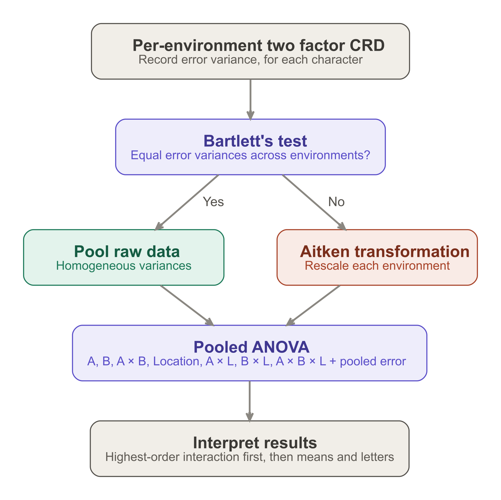
RAISINS runs the individual analyses, performs Bartlett’s test separately for every character, applies the Aitken transformation only to the characters that need it, assembles the pooled ANOVA under the model you selected, and attaches letter groupings, all from a single click of Run Analysis. The flowchart is here so you understand why the software did what it did, not because you must do it yourself.
4 Assumptions of a pooled two factor CRD
A pooled 2FCRD inherits the assumptions of the ordinary two factor CRD and adds one of its own, homogeneity of error variance across environments.
| Assumption | What it means | What if it fails? |
|---|---|---|
| Randomisation | Within each environment, all treatment combinations are assigned to experimental units completely at random | Serious. Settled by good design, not fixable at the analysis stage |
| Independence | Each observation is unrelated to the others | Handled by design and randomisation |
| Normality | Errors within each environment are approximately normal | Try a log, square-root, or arcsine transformation (Section 11) |
| Homogeneity of variance across environments | Each environment’s error variance is roughly the same | RAISINS checks this with Bartlett’s test and applies the Aitken transformation automatically when it fails (Section 12) |
| A complete factorial in every environment | Every level of Factor A appears with every level of Factor B, in every environment | An incomplete crossing leaves interaction terms unestimable; fix the layout before analysing |
| Continuous response | The measurement is a proper number (yield, weight, concentration), not a category | Use a method designed for that data type instead |
The one assumption unique to pooling, equal error variance across environments, is the one you do not have to police yourself. RAISINS tests it for every character and repairs it where needed, before it builds the pooled ANOVA. Your job is to design each environment’s factorial well, keep the crossing complete, and randomise properly; RAISINS handles the rest.
5 Getting to the module
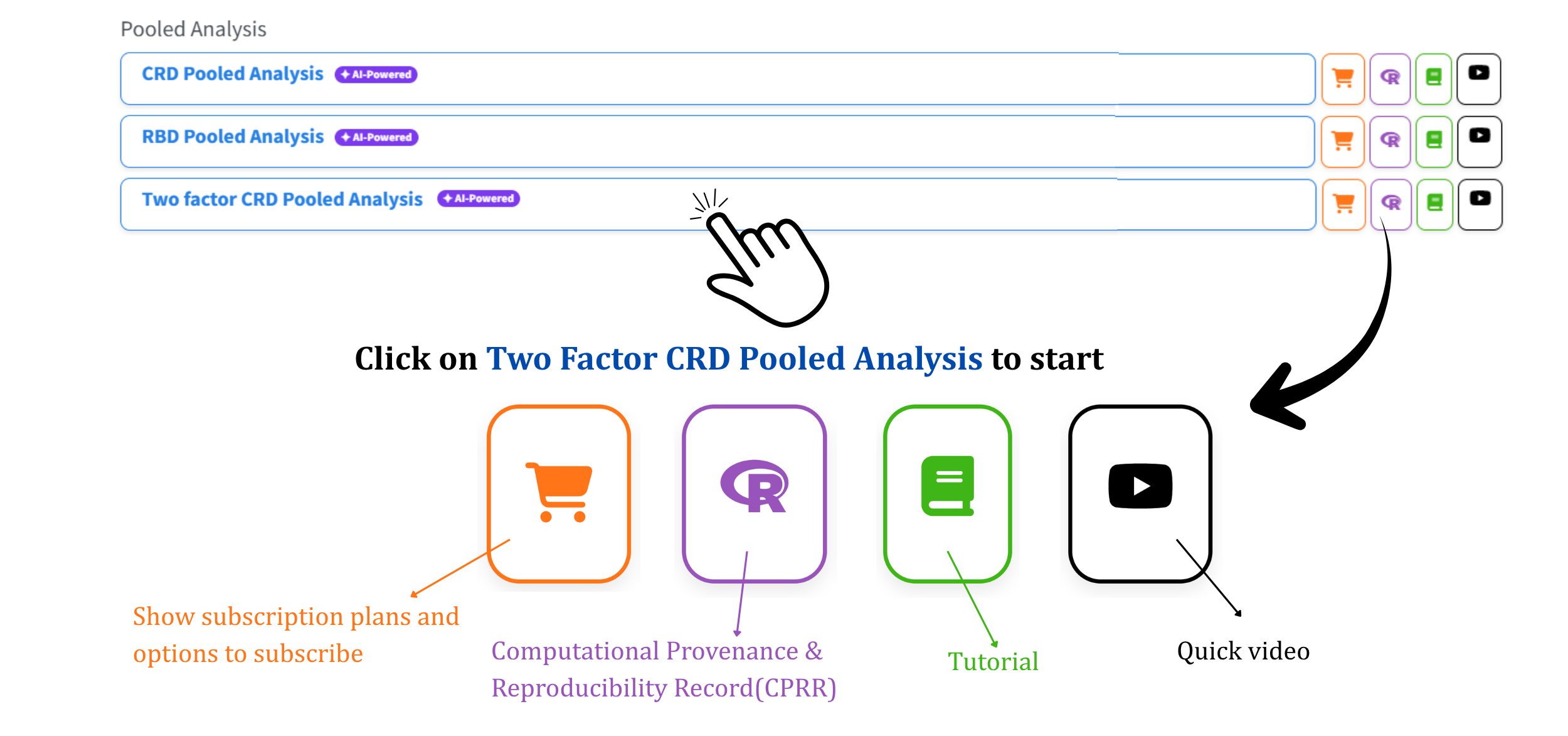
Now that the theory is clear, let us run the analysis. Visit the RAISINS home page at www.raisins.live and go to Data Analysis. Under Pooled Analysis you will find three entries, CRD Pooled Analysis, RBD Pooled Analysis, and Two factor CRD Pooled Analysis. Click the third to start, as shown in Figure 2.
5.1 Computational Provenance & Reproducibility Record
CPRR (Computational Provenance & Reproducibility Record) provides a transparent and comprehensive record. Click the CPRR icon shown in Figure 2 to access it and know about the computational workflow performed during the analysis. The record for this module states the R version and the exact version of every package used, and names the specific function behind each reported result. CPRR lists every default parameter and decision rule applied by the module and provides fully runnable R code that reproduces each analytical step. Users can execute the code in R to independently reproduce and verify the results. It carries its own DOI.
To cite the platform itself in a paper, thesis, or report, use the RAISINS citation, available in APA, Harvard, and BibTeX formats at www.raisins.live/citation.html. That is the primary reference, and for most manuscripts it is all you need.
The CPRR for the Pooled Analysis in Two Factor CRD module is at www.raisins.live/module_record/pooled_2fcrd.html.
Cite the RAISINS paper as your primary reference for the platform. Add the CPRR as supporting documentation when a journal asks for details of the computing environment, or when you want your methods section to be precise about versions and functions rather than saying “analysis was carried out using an online tool.” The CPRR supports the citation and ensures computational reproducibility.
6 Preview mode and Quick Tour
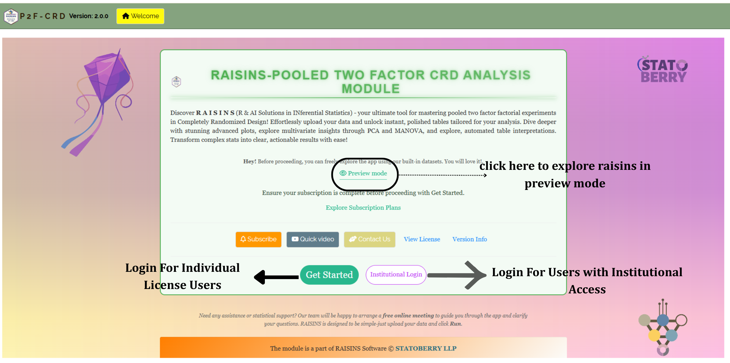
Before subscribing, you can explore the entire module using Preview mode, reached from the welcome page shown in Figure 3 by clicking the Preview mode link. Preview mode loads built-in datasets so you can try every feature (the pooled ANOVA, the Bartlett test, both plot tabs, the per-character ANOVA, the multivariate index, and the RA-One assistant) without uploading your own data. The same page offers Get Started for individual-licence users and Institutional Login for institutional access. First-time users are also offered a Quick Tour, an interactive, step-by-step walkthrough that highlights each control and explains what it does. You can retake the tour at any time from the Quick Tour tab in the green navigation bar.
This module has two levels of navigation and it helps to notice them early. The green bar at the very top carries Analysis, Create Data, Datasets, RA-One, User, and Quick Tour, these are the app-wide tabs, and the module version (2.0.0) is printed beside the P2F-CRD logo. The second row, inside the Analysis page itself, carries Analysis Results, Basic Plots, Advanced Plots, AI interpretation, Indv. ANOVA, Multivariate, FAQs, and View Data, these are the outputs of your analysis. Almost everything in this tutorial happens on that second row.
7 A working example
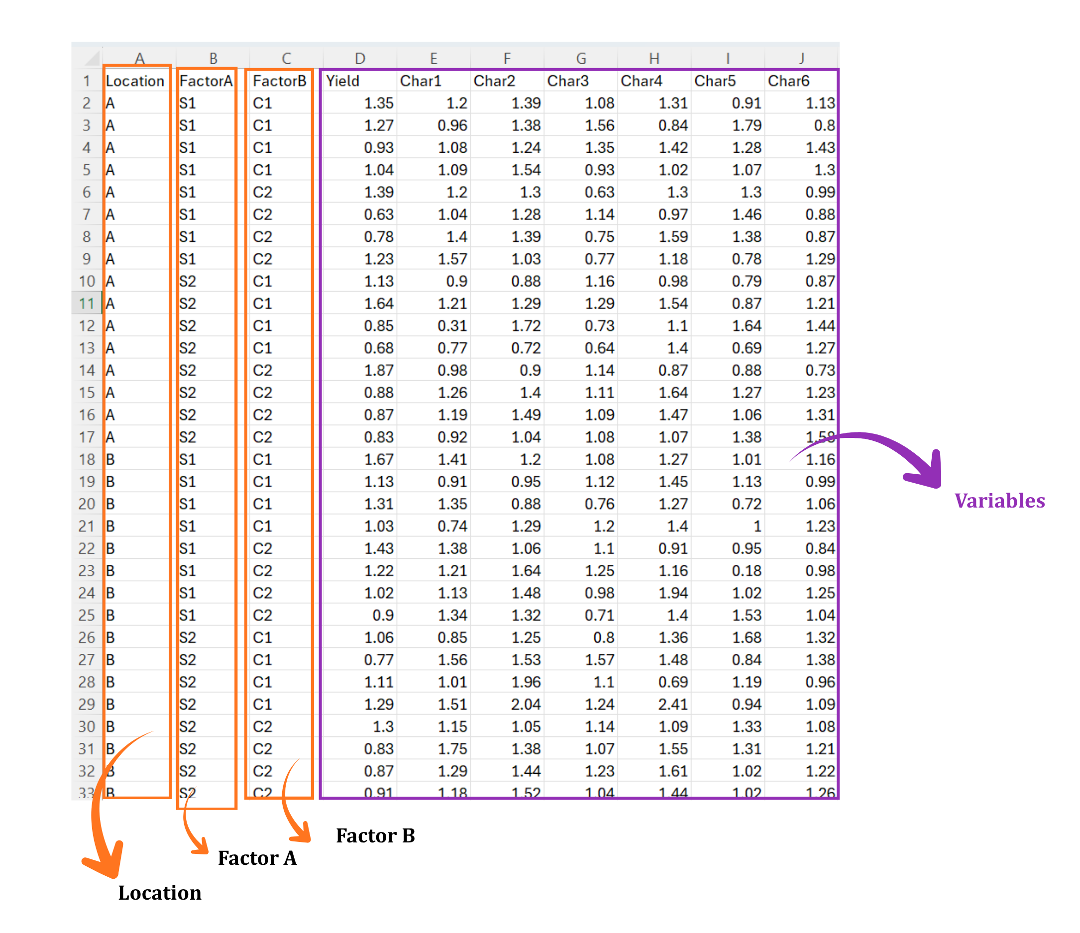
This tutorial uses the module’s own demonstration dataset. Two factors were crossed: FactorA with two levels, S1 and S2, and FactorB with two levels, C1 and C2. The resulting four treatment combinations were laid out as a completely randomized design and replicated four times, and the entire factorial was repeated at two locations, A and B. That gives 2 × 2 × 4 × 2 = 32 observations, and eight Location × FactorA × FactorB combinations in all.
Seven response variables were recorded on every unit: Yield, Char1, Char2, Char3, Char4, Char5, and Char6. This illustrates one of the module’s real conveniences, several characters are analysed in a single run, each pooled independently and each getting its own Bartlett test, its own ANOVA, and its own means tables. Figure 4 shows the layout.
Because the characters behave differently. In this dataset Yield turns out completely non-significant, Char1 shows a Factor B effect, Char2 shows interactions, and Char6 fails Bartlett’s test and has to be repaired before pooling. A single-trait example would show you one path through the module; this one shows you nearly all of them.
8 How to prepare your data
Your analysis is only as good as your data. Feed RAISINS high-quality data and it will deliver powerful insights; feed it messy data and the results will not be trustworthy. You have four routes:
- Create your dataset in MS Excel
- Build your dataset directly within the RAISINS app
- Using the Model datasets in RAISINS as a reference
- Create your dataset using the RA-One chat assistant
8.1 Preparing data in MS Excel
Open a new blank sheet in MS Excel containing only one sheet, and avoid adding any unnecessary content. The dataset should follow a column-based format with a clear structure for a pooled two factor CRD:
- The first column holds the environment label, the location or season (e.g. “A”, “B”).
- The second column holds the levels of Factor A (e.g. “S1”, “S2”).
- The third column holds the levels of Factor B (e.g. “C1”, “C2”).
- Every response variable under study (e.g. Yield, Char1, Char2) occupies its own separate column.
Each environment label repeats for every observation recorded in it, and within each environment every combination of Factor A and Factor B repeats according to the number of replications. Note that there is no replication column, a CRD has no blocking, so the replicates are simply repeated rows of the same combination. The file can be saved as CSV, XLS, or XLSX, but CSV is recommended as it is lighter and loads faster. Ensure there are no unwanted spaces in the column names or in the labels. For reference, see the structure in Figure 4.
Dataset creation rules
- Column naming convention
- No spaces allowed in column names.
- Use underscores (
_) or full stops (.) for separation. - Avoid symbols and special characters such as %, #.
- Data arrangement
- Start the data towards the upper-left corner.
- Ensure the row above the data is not blank.
- Keep the environment column first, Factor A second, and Factor B third.
- Cell management
- Avoid typing or deleting in cells without data.
- If needed, select the affected cells, right-click, and choose Clear Contents.
- Balance and completeness
- Every level of Factor A must appear with every level of Factor B, in every environment.
- Keep the number of replications consistent so the design stays balanced.
- Labels
- Keep the spelling and capitalisation of the environment and factor labels perfectly consistent throughout each column, “S1” and “s1” would be read as two different levels.
How to save as CSV in MS Excel
Open your workbook. Ensure your data is arranged properly with only one sheet.
Click the ‘File’ menu. Go to the top-left corner and click File.
Choose ‘Save As’ or ‘Save a Copy’. Select the location where you want to save your file.
Set file type to CSV. In the ‘Save as type’ dropdown, choose CSV (Comma delimited) (*.csv).
Name your file. Enter a relevant file name without spaces (use underscores if needed).
Click ‘Save’. Click Save to export the file.
💡 Tip: Before saving, double-check that your data is on the first sheet and follows the required format: no empty rows above the data, meaningful column names, an environment column, two factor columns, and one column per response variable.
8.2 Prepare using Create Data in RAISINS
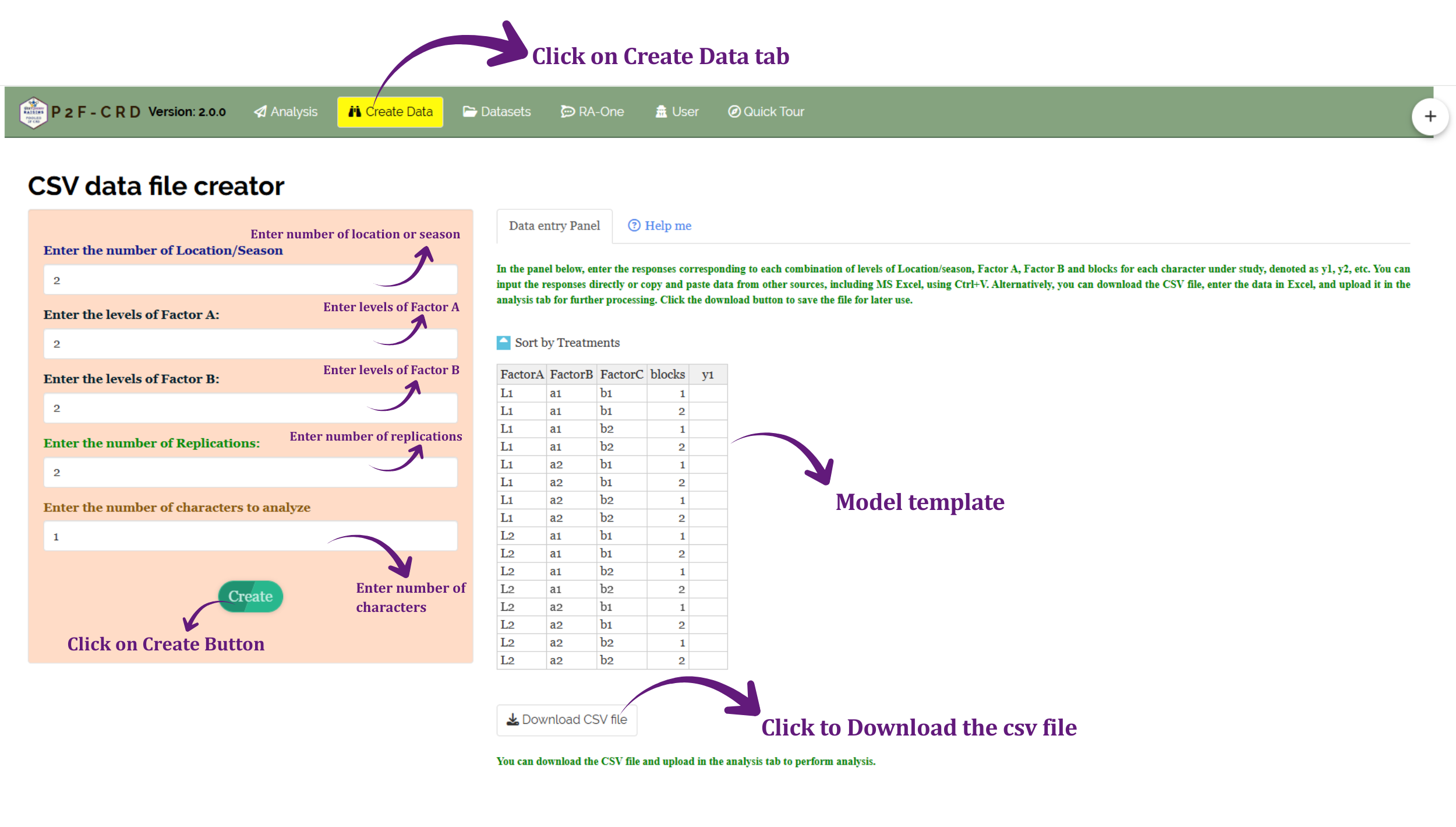
If you are unsure about the correct format, do not worry, RAISINS can create the data layout for you using the prescribed template. Head to the Create Data tab in the green bar, where the CSV data file creator asks five questions:
- Enter the number of Location/Season (environments)
- Enter the levels of Factor A
- Enter the levels of Factor B
- Enter the number of Replications
- Enter the number of characters to analyze
Then click Create. The model template appears on the right, one row for every Location × Factor A × Factor B × replication combination, with an empty response column (y1, y2, …) for each character you asked for (Figure 5). You can type the observations straight into the panel, or paste them in from Excel with Ctrl+V. When you are done, click Download CSV file and upload the saved file on the Analysis tab.
8.3 Download Model Datasets
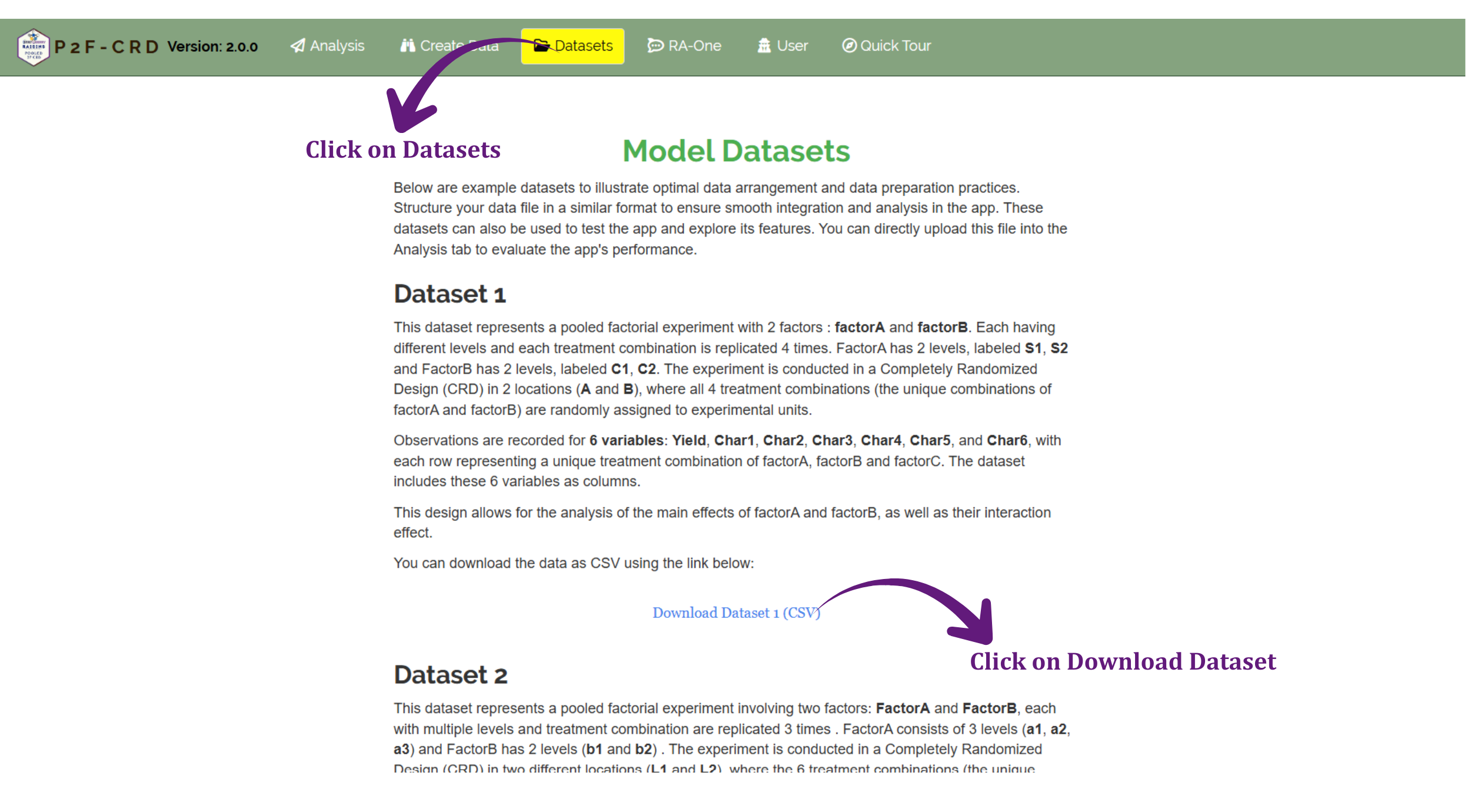
If you are unsure about the required data format or would like to explore the module before using your own data, RAISINS provides model datasets for reference under the Datasets tab. Each is described in plain language before you download it, Dataset 1 is the 2 × 2 factorial in two locations with four replications used throughout this tutorial, while Dataset 2 is a 3 × 2 factorial replicated three times across two locations, so you can see how the tables grow when a factor gains a level. To use them:
- Navigate to the Datasets tab
- Read the description to find the layout closest to your own experiment
- Click the Download Dataset (CSV) link beneath it
- Save the file, then either study it as a template or upload it directly to explore the analysis
8.4 Creating a dataset using RA-One chat
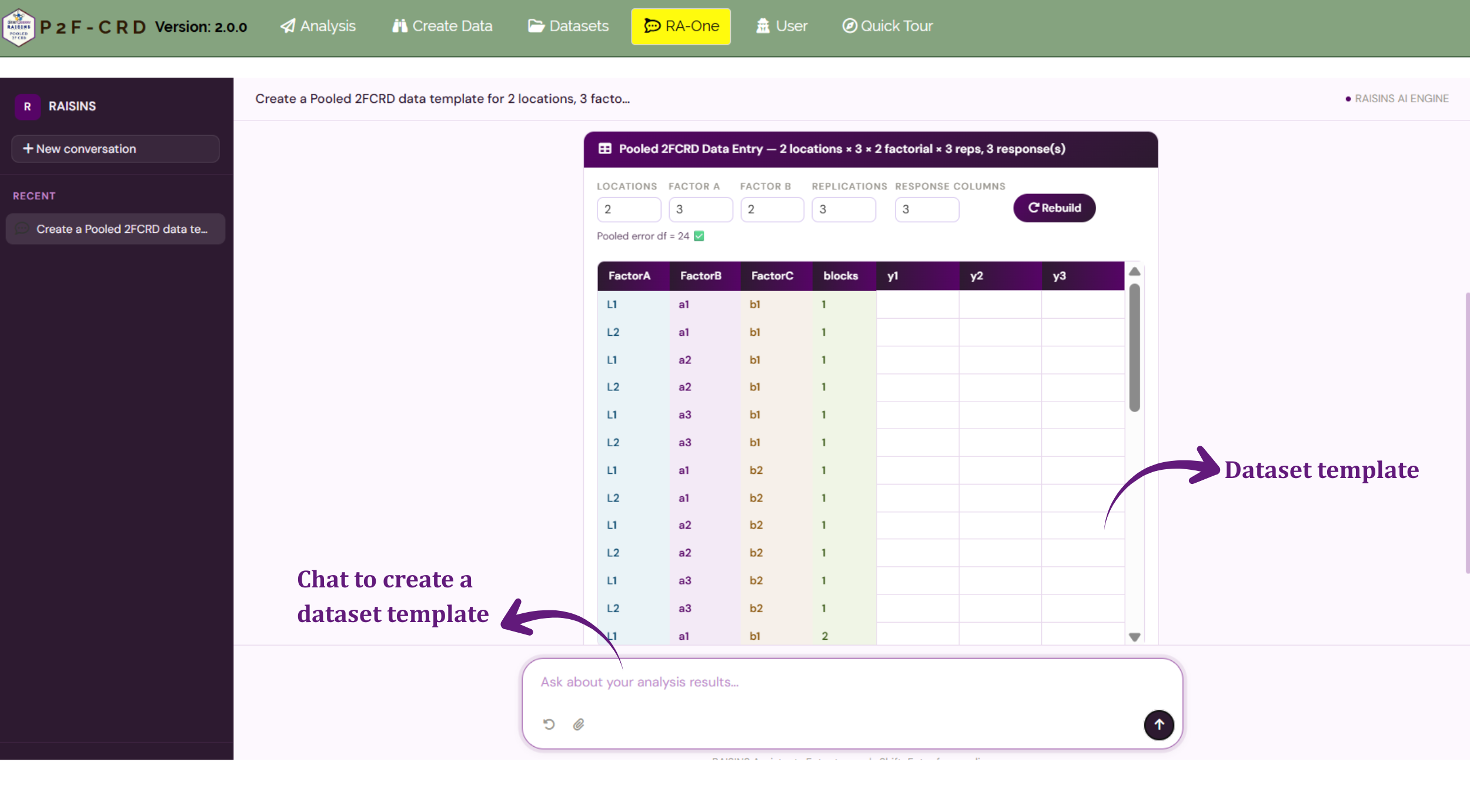
RA-One, the built-in chat assistant, can build a correctly formatted dataset through a plain-language conversation. Open the RA-One tab in the green bar and describe the experiment you ran, for example “Create a Pooled 2FCRD data template for 2 locations, 3 levels of Factor A, 2 levels of Factor B, 3 replications and 3 responses.” RA-One replies with a live data-entry grid rather than a static block of text (Figure 7). The grid has editable boxes for LOCATIONS, FACTOR A, FACTOR B, REPLICATIONS, and RESPONSE COLUMNS, so you can change your mind and press Rebuild without retyping the request.
Two details on that panel are worth noticing. It prints the resulting pooled error df with a green tick, a quick sanity check that your design has enough replication to estimate the error, and it lays the rows out with every combination of the factors already filled in, leaving only the response columns (y1, y2, y3) blank for you. Fill them in, download the CSV, and upload it under Analysis Results.
9 The Analysis Results tab
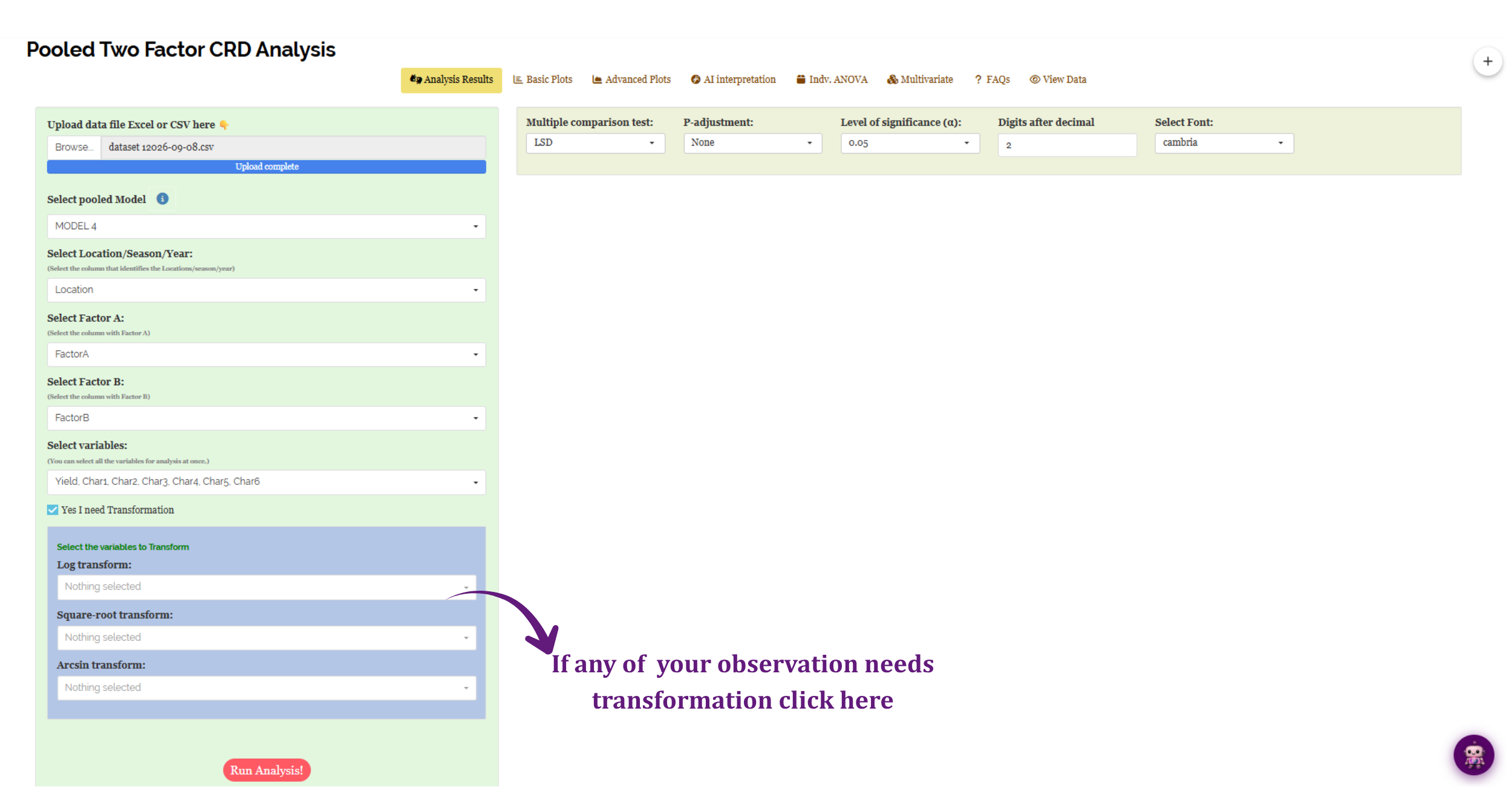
Figure 8 shows the Analysis Results tab in detail. Upload your prepared file by clicking Browse in the green sidebar and wait for the blue Upload complete bar. Five selectors then appear, and they must be answered in order:
- Select pooled Model — the structural question of Section 10, whether your factors and environments are fixed or random.
- Select Location/Season/Year — the column that identifies the environments.
- Select Factor A — the column holding the first factor.
- Select Factor B — the column holding the second factor.
- Select variables — the response columns. You can select all of them at once, and in the working example all seven (Yield, Char1 … Char6) are analysed in a single run.
Below these sits a Click for Transformation checkbox (Section 11), and then the pink Run Analysis! button. Once clicked, every output becomes available across the sub-tabs: Analysis Results, Basic Plots, Advanced Plots, AI interpretation, Indv. ANOVA, Multivariate, FAQs, and View Data.
The olive strip along the top of the results panel holds five display controls that you can change at any time without re-running: the Multiple comparison test (LSD, Tukey’s HSD, or DMRT), the P-adjustment, the Level of significance (α), the Digits after decimal, and the Select Font used in the tables. In the working example these were left at LSD, no P-adjustment, α = 0.05, two decimals, and the Cambria font.
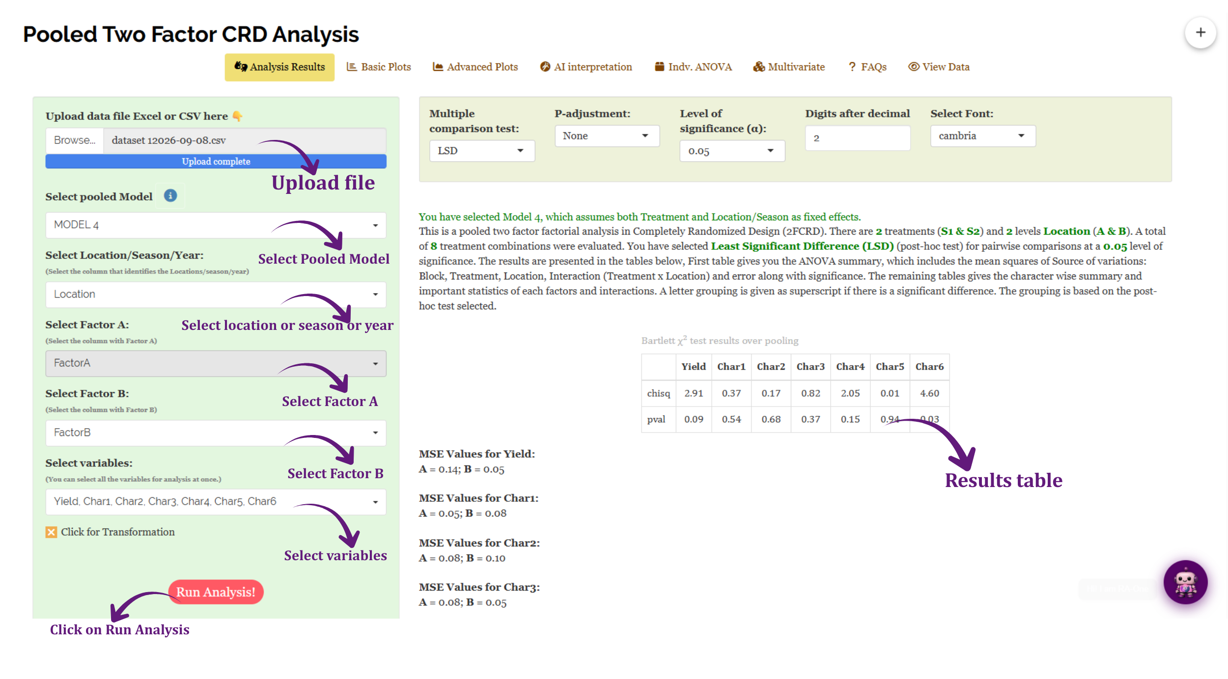
The first thing RAISINS prints after a successful run is a green paragraph restating, in plain English, exactly what it just did. For the working example it reads: “You have selected Model 4, which assumes both Treatment and Location/Season as fixed effects. This is a pooled two factor factorial analysis in Completely Randomized Design (2FCRD). There are 2 treatments (S1 & S2) and 2 levels Location (A & B). A total of 8 treatment combinations were evaluated. You have selected Least Significant Difference (LSD) (post-hoc test) for pairwise comparisons at a 0.05 level of significance.” Read that sentence before you read any number. It is the cheapest way to catch a mis-assigned column, if the environment and a factor have been swapped in the dropdowns, this paragraph will say so.
Which multiple-comparison test should I pick?
LSD (Least Significant Difference) is the default and the most sensitive, it declares two means different as soon as they differ by more than the critical difference. It is a good general choice for a well-designed trial.
Tukey’s HSD (Honestly Significant Difference) is more conservative and controls the error rate across all pairwise comparisons at once, a safer choice when you have many treatment combinations and want to guard against false positives. In a pooled 2FCRD the combination table can grow quickly (levels of A × levels of B × environments), so HSD is worth considering here more often than in a simple one-factor design.
DMRT (Duncan’s Multiple Range Test) sits between the two and is traditional in agricultural research.
All three produce the same kind of letter grouping; they differ only in how strict the cut-off is. When in doubt, LSD is a reasonable default, and RAISINS lets you switch and re-read instantly.
10 Choosing a pooled model
Before it reports a single number, the module asks one structural question: are your treatments and your environments fixed things you chose deliberately, or a random sample of a larger population? The answer changes which error term each effect is tested against, and RAISINS lets you state it explicitly through the Select pooled Model control. There are four choices:
| Model | Treatment | Location / Season | Read it as |
|---|---|---|---|
| Model 1 | random | random | Both the treatment combinations and the environments are samples of larger sets |
| Model 2 | fixed | random | You care about these specific factor levels, tested across a random sample of environments |
| Model 3 | random | fixed | You care about these specific environments, testing a random sample of factor levels |
| Model 4 | fixed | fixed | Both the factor levels and the environments are the only ones you care about |
In the working example Model 4 was selected, treating both the factors and the locations as fixed effects. That is the right choice when the two locations are themselves the objects of study, say your own two research stations, rather than a sample standing in for a wider region. If instead your locations were picked to represent a growing region you hope to generalise to, Model 2 is the usual choice, because it treats the environment as random and makes the factor × Location interactions the natural yardstick for judging whether an effect travels.
Whichever you choose, RAISINS states your selection in plain language at the top of the results (Figure 8) so there is never any doubt about which model produced the numbers below.
Under a fully fixed model like Model 4 every effect is tested against the pooled error, which is what you see in the ANOVA of Figure 10, each F is that row’s mean square divided by the pooled error mean square. Under a mixed model the denominators change: a random environment makes the corresponding interaction the correct yardstick for the main effect above it, so the same data can produce different F values and different p-values under Model 2 than under Model 4. This is not the software being inconsistent, it is the model answering a different question. Decide which one matches your sampling scheme before you look at the p-values, not after.
11 Transformation
Two distinct kinds of transformation live in this module, and it helps to keep them apart.
The Aitken transformation is applied automatically and only when Bartlett’s test finds the error variances unequal across environments for a given character (Section 12). You do not choose it; RAISINS applies it for you, character by character, exactly where the data demand it.
The normalising transformations, logarithmic, square-root, and arcsine, are ones you apply manually when a character is not normally distributed. Tick Click for Transformation in the sidebar and the panel expands into three dropdowns, Log transform, Square-root transform, and Arcsin transform, as shown in Figure 9. Each dropdown takes a list of variables, so you can log one character, square-root another, and leave the rest untouched in the same run.
Logarithmic transformation converts a skewed distribution into a more symmetrical one by replacing each data point \(x\) with its logarithm. It is applied to positive, continuous data where the variance grows in proportion to the mean, a pattern common in phenomena that grow multiplicatively.
Square root transformation stabilises variance and reduces right-skewness by replacing each data point \(x\) with \(\sqrt{x}\). It is primarily used for non-negative count data, such as those following a Poisson distribution, where variance increases with the mean.
Arcsine transformation (the angular transformation) is designed for proportions or percentages bounded between 0 and 1. By taking \(\arcsin(\sqrt{p})\) it stretches the ends of the distribution near 0 and 1, where variance is naturally small.
It is tempting, on seeing a significant Bartlett test, to log the offending character and re-run. Resist it. Bartlett’s test is about unequal variance between environments, and that is precisely what the Aitken transformation exists to repair, automatically and without you doing anything. The manual transformations here are for a different problem, non-normality within an environment. Applying one to chase a Bartlett p-value changes the scale your means are reported on for no good reason.
After choosing any transformation, proceed to Section 12 and Section 13 for the analysis.
12 Homogeneity of variance and the Aitken transformation
The whole point of a pooled analysis is to combine several experiments into one. But you are only allowed to pool them if the experiments are measuring on comparable terms, specifically, if the error variance is roughly the same in every environment. If one location is far noisier than the others, throwing all the data into a single error term would let that one messy location contaminate every comparison in the study. So before pooling, RAISINS runs Bartlett’s test on each response variable across the locations, and prints the result at the top of the Analysis Results panel (Figure 8).
Bartlett’s test takes the error variance (the MSE) from each location’s individual two factor CRD and asks whether they are all equal. Its null hypothesis is that the variances are homogeneous. A large p-value (≥ 0.05) is the “good” outcome here, it means the variances are compatible and the experiments may be pooled directly. A small p-value (< 0.05) means at least one location wobbles by a different amount, and that character must be re-scaled before pooling.
Table 1: Bartlett χ² test for homogeneity of error variances across locations
| Statistic | Yield | Char1 | Char2 | Char3 | Char4 | Char5 | Char6 |
|---|---|---|---|---|---|---|---|
| χ² | 2.91 | 0.37 | 0.17 | 0.82 | 2.05 | 0.01 | 4.60 |
| p-value | 0.09 | 0.54 | 0.68 | 0.37 | 0.15 | 0.94 | 0.03 |
12.1 Interpretation from Table 1
Six of the seven characters pass comfortably. Char5 is the most homogeneous of all (χ² = 0.01, p = 0.94), meaning its two locations produced almost identical error variances, and Char1, Char2, Char3, and Char4 are all well clear of the threshold. Yield sits closest to the line without crossing it (χ² = 2.91, p = 0.09): a little uneven, but not enough to reject homogeneity at α = 0.05, so it is pooled as it stands.
Char6 fails (χ² = 4.60, p = 0.03). Its error variance genuinely differs between location A and location B, so RAISINS applies the Aitken transformation to Char6 and to Char6 alone, before building its pooled ANOVA. The other six characters are left completely untouched. The module states this explicitly in the AI interpretation (Section 17): “For character(s): Char6 Aitken transformation is applied as Bartlett’s test was significant. For remaining characters, no transformation was applied as variance was homogeneous across all Location.”
Beneath the Bartlett table the module prints the raw ingredient of that decision, the MSE of each location, for each character. For Yield these are A = 0.14 and B = 0.05, a near threefold gap that explains why Yield’s χ² is the second largest in the table. For Char1 they are A = 0.05 and B = 0.08, for Char2 A = 0.08 and B = 0.10, and for Char3 A = 0.08 and B = 0.05, all close enough to pool without complaint. Reading these MSE values is the quickest way to see which environment is the noisy one when a character does fail.
For a character that fails Bartlett’s test, RAISINS divides each location’s observations by the square root of that location’s own MSE. This puts every environment on an equal-variance footing, so that a noisy location no longer shouts louder than a quiet one in the pooled error term. The transformed values then carry through the ANOVA, and where means are reported the transformed mean appears in parentheses beside the original. The repair is silent, automatic, and applied only to the offending character, you never lose the ability to pool, RAISINS simply fixes the scale first.
Because Char6 was Aitken-transformed, every significance decision about Char6, its F values, its p-values, and its letter groupings, was made on the transformed data. This is the correct thing to do, but it means you can occasionally see two Char6 means that look almost identical on the original scale carrying different letters. The letters are right; the original-scale means are simply not the numbers the test was performed on. Whenever you quote a Char6 result in a report, say that an Aitken transformation was applied.
13 The pooled ANOVA
With the homogeneity question settled, RAISINS builds the pooled analysis of variance. This is the heart of the module. Instead of two separate factorial tables, one per location, you get a single table that partitions the total variation into the seven sources of Section 2 plus a pooled error, and tests each one.
Each character gets its own table, reached from the Indv. ANOVA tab through the Select Character dropdown (Figure 10). Pick a character from the list and its full pooled ANOVA appears beside it, with a footnote block reminding you that * marks significance at the 5% level, ** at the 1% level, and NS non-significant.
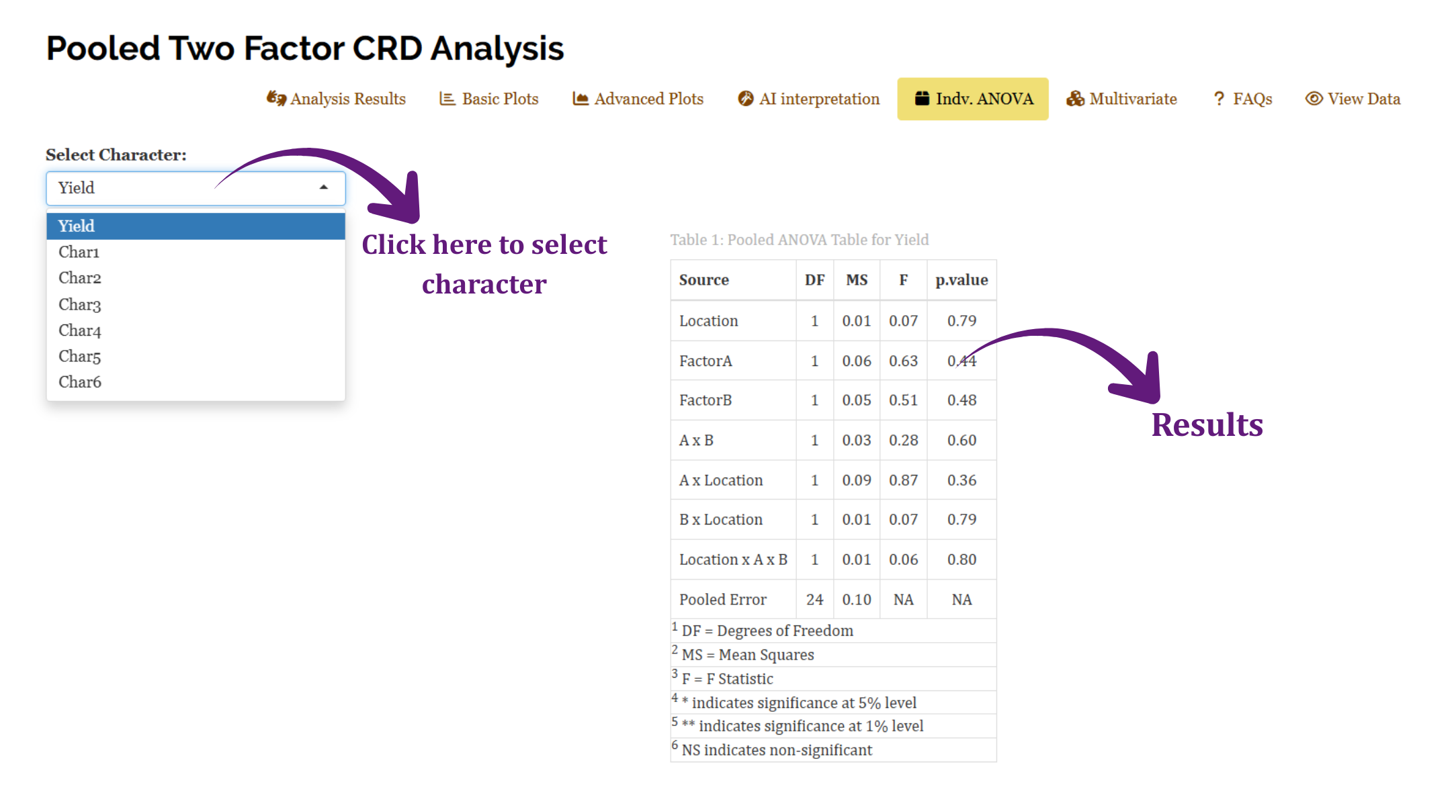
Table 2: Pooled ANOVA for Yield
| Source of variation | DF | MS | F | p-value |
|---|---|---|---|---|
| Location | 1 | 0.01 | 0.07 | 0.79 |
| FactorA | 1 | 0.06 | 0.63 | 0.44 |
| FactorB | 1 | 0.05 | 0.51 | 0.48 |
| A × B | 1 | 0.03 | 0.28 | 0.60 |
| A × Location | 1 | 0.09 | 0.87 | 0.36 |
| B × Location | 1 | 0.01 | 0.07 | 0.79 |
| Location × A × B | 1 | 0.01 | 0.06 | 0.80 |
| Pooled Error | 24 | 0.10 |
13.1 Interpretation from Figure 10
Start with the degrees of freedom, because they are a free check on your design. Every effect carries 1 degree of freedom, which is exactly right for a two-level factor crossed with a two-level factor across two locations: each source has (levels − 1) = 1. The Pooled Error carries 24 df, and the eight rows sum to 31, one less than the 32 observations. If those numbers do not match your own design, the columns were assigned wrongly and nothing below is worth reading.
Now the substance: for Yield, nothing is significant. Every p-value sits between 0.36 and 0.80, and every mean square (0.01 to 0.09) is smaller than the pooled error mean square of 0.10. That last observation is the crux, an F statistic is the row’s mean square divided by the error mean square, so a mean square below the error produces an F below 1 and there is no evidence of an effect at all. The largest F in the table, A × Location at 0.87, is still under 1.
The honest reading is that Yield did not respond to spacing, to compost, to their combination, or to location, and none of those answers changed between the two locations. Every ladder rung of Section 2 is clear, so you may quote the main effects safely, and the main effects say there is nothing to quote. That is a real result, not a failed analysis: for this character the treatments simply did not move the needle.
A table of NS rows means your experiment did not detect a difference; it does not prove the treatments are identical. With four replications per combination at each of two locations, only fairly large effects would show up. If a null result matters to your conclusion, report the size of the difference you could have detected alongside the p-value, rather than writing “the treatments had no effect.”
Switching the Select Character dropdown walks you through the other six characters, and they are not all as quiet as Yield. Across the full set the module found significant effects for three of them, summarised in Section 14, and it is worth stepping through each character in turn rather than reading only the first table you are shown.
14 Means, groupings and the summary tables
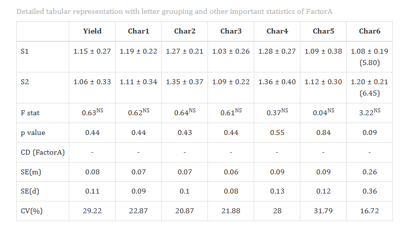
The ANOVA tells you whether an effect exists; it never tells you which level beat which. That is the job of the multiple-comparison test chosen in the sidebar, which attaches letter groupings to the means: levels sharing a letter are not significantly different, levels with different letters are. Beneath the ANOVA summary the Analysis Results tab prints a character-wise summary table for each of the seven sources that can carry means, so you get a means table for Factor A, one for Factor B, one for the A × B combinations, one for Location, and one for each of the three interactions involving Location.
Crucially, RAISINS only attaches letters where the ANOVA earned them. If a source is non-significant for a character, no post-hoc test is run for it and the critical difference is deliberately left blank, so you are never invited to read into differences that are statistically indistinguishable. This is why most of the tables in the working example are letter-free.
14.1 What the working example actually found
Reading across all seven characters, the module reports significance in only three places, and each one illustrates a different rung of the ladder in Section 2.
Factor A produced nothing. No character showed a significant Factor A main effect, so no pairwise comparison was performed for it and every Factor A table is letter-free. The same is true of the A × B interaction and of B × Location: neither was significant for any character.
Factor B mattered for Char1 (p = 0.05). Here C2 has the highest mean (1.25 ± 0.21) and C1 the lowest (1.05 ± 0.32), and with only two levels in play they are of course significantly different from one another. Because no interaction involving Factor B was significant for Char1, this main effect is safe to quote on its own: for Char1, C2 outperforms C1, and it does so at both locations.
Location mattered for Char6 (p = 0.00), with A highest (1.15 ± 0.26) and B lowest (1.13 ± 0.15). Remember that Char6 is the character that failed Bartlett’s test and was Aitken-transformed (Section 12) — the test was carried out on the transformed scale, which is why two original-scale means this close can separate cleanly.
Char2 is the interesting one, and the only character where the ladder bites. Its Location × Factor A interaction is significant (p = 0.04), with S2 × B highest (1.52 ± 0.33) and S2 × A lowest (1.18 ± 0.35); note that S2 occupies both ends, which is the signature of an effect that reverses between environments. Its Location × A × B interaction is significant too (p = 0.04), with S2 × C1 × B highest (1.70 ± 0.37) and S1 × C1 × B lowest (1.08 ± 0.20).
For Char2 the plain A × B interaction was not significant, yet Location × A × B was. That combination is not a contradiction, it is the whole reason the pooled design exists. Averaged across the two locations the factorial interaction cancels out to nothing; within each location separately it is real, and it points in different directions at A and at B. Quoting an overall “best combination” for Char2 would average away the very effect the experiment found. For this character you must report the results location by location, not pooled.
Notice also how the “on par” language in the module’s own interpretation (Figure 15) works. For the Char2 combination table it says that S2 × C1 × B is on par with S1 × C1 × A, S1 × C2 × B and S2 × C2 × B, because those means share at least one letter, and that the lowest combination, S1 × C1 × B, is on par with six of the other seven. With eight combinations, four replications each and a fair amount of noise, only the two extremes are cleanly separated, everything in between overlaps. That is normal, and it is a more honest picture than a ranking that pretends all eight are distinguishable.
A glossary of the result-table rows
Mean ± SD — each cell is the average of that factor level (or combination) followed by its standard deviation. Where an Aitken transformation was applied, as for Char6, the transformed mean is shown in parentheses.
Letter grouping (a, b, c) — attached as a superscript by the multiple-comparison test. Means sharing a letter are not significantly different at the chosen α; means with different letters are. Two treatments described as “on par” are simply two treatments sharing a letter.
F stat — the ratio testing whether that source’s means differ, equal to the source’s mean square divided by the pooled error mean square under a fixed-effects model. The asterisks (* 5%, ** 1%, NS not significant) come straight from this statistic.
CD (Critical Difference) — the smallest gap between two means that counts as significant. Left blank whenever the corresponding effect is non-significant, which in this dataset is most of the time.
SE(m) — the standard error of a single mean. SE(d) — the standard error of the difference between two means, the quantity the CD is built from.
CV (%) — the coefficient of variation, the pooled error expressed as a percentage of the grand mean. It is a measure of experimental precision: lower is tighter. MSE and CV(%) are common for the whole experiment, since the pooled analysis uses one common error term.
RAISINS decides the letter groupings using the full-precision CD and prints a CD rounded to the number of decimals you chose in the Digits after decimal box. Occasionally two means that look closer together than the printed CD still receive different letters, because the grouping used more decimal places than the display shows. The letters are always the authoritative statement of significance.
15 Basic and Advanced Plots
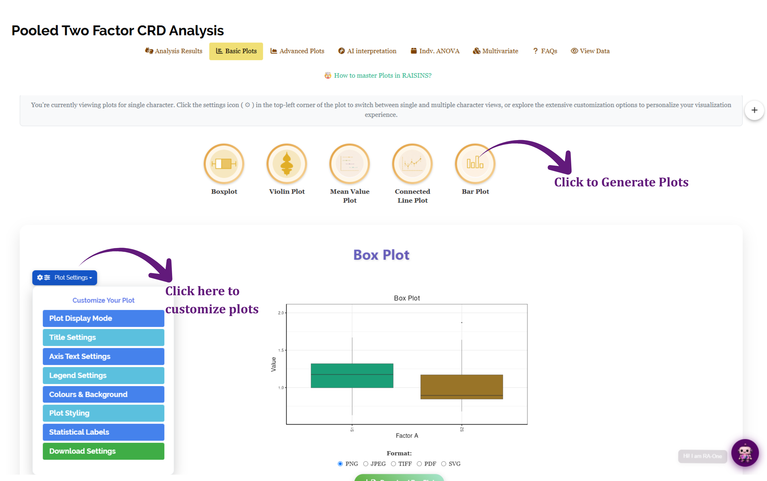
Numbers convince, but a picture persuades. Two dedicated tabs turn your results into publication-ready graphics, and both work the same way: click an icon to generate the plot, then open the blue Plot Settings dropdown on the left to customise it.
The Basic Plots tab (Figure 12) offers five plots, a Boxplot, a Violin Plot, a Mean Value Plot, a Connected Line Plot, and a Bar Plot. The settings panel groups the controls into Plot Display Mode (switch between viewing a single character and several at once), Title Settings, Axis Text Settings, Legend Settings, Colours & Background, Plot Styling, Statistical Labels, and Download Settings. Beneath every plot sits a Format selector offering PNG, JPEG, TIFF, PDF and SVG, so you can take a raster image for a slide or a vector file for a journal. The box plot in Figure 12 is drawn by Factor A, showing the S1 and S2 distributions side by side.
Under Statistical Labels you can print the letter groupings from Section 14 directly onto the plot. A bar chart carrying its own a/b/c superscripts is worth a paragraph of explanation in a results section, and it keeps the figure consistent with the table beside it. Turn it on before you export anything for publication.
The Advanced Plots tab (Figure 13) goes considerably further, with twelve plots arranged in two rows: Interaction Plot, Interaction Plot II, Summary Plot, Raincloud Plot, Advanced Raincloud Plot, Circular Plot, QQ Plot, Distribution Plot, Pair Plot, Correlation Plot, 3D Scatter Plot, and 3D Scatter + Line. Its settings panel is organised slightly differently, into Title & Axes, Error Bars, Line & Point, Colours & Theme, Axis Text, Legend, Plot Styling, and Download Settings.
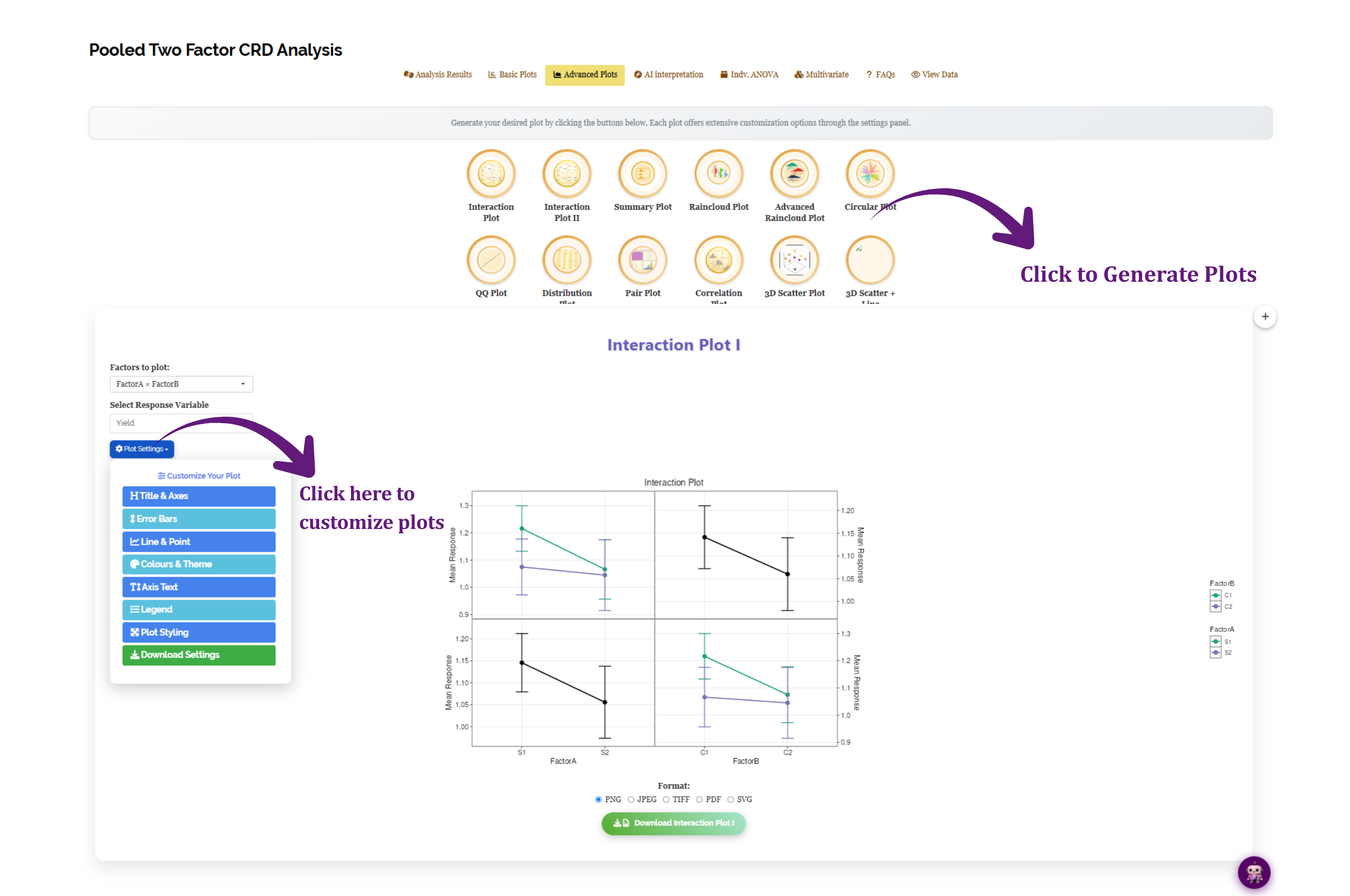
Of the twelve, the two Interaction Plots are the ones this design was built for. Each has a Factors to plot dropdown, set to FactorA × FactorB in Figure 13, and a Select Response Variable dropdown, set to Yield. The plot then draws mean response against one factor with a separate line per level of the other, complete with error bars. Read it by asking one question: are the lines parallel? Parallel lines mean no interaction, the effect of one factor is the same at every level of the other. Lines that converge, diverge or cross mean an interaction, and crossing lines mean a reversal. Switch the dropdown to a Location pairing and the same picture answers the far more important question of whether your effect survives a change of environment. For Char2, which showed a significant Location × Factor A interaction (Section 14), this is exactly the plot that makes the reversal visible.
The remaining plots serve the checks around the analysis rather than the analysis itself. The QQ Plot and Distribution Plot let you inspect the normality assumption of Section 4 before you trust a p-value. The Pair Plot and Correlation Plot show how the seven characters move together, which is the natural preparation for the multivariate index (Section 16). The Raincloud plots combine a distribution, a box and the raw points in one figure, and the 3D views let you look at three characters at once.
16 Multivariate: the PCA index score
So far each character has been judged on its own. But a combination that is best for Char1 might not be best for Char2, and in a real recommendation you usually want a treatment that performs well across all characters at once. The Multivariate tab handles this with Principal Component Analysis (PCA). Click Click here for PCA Index and the module reduces your characters to a set of underlying components and builds a single index score for each treatment combination, ranking them (Figure 14).
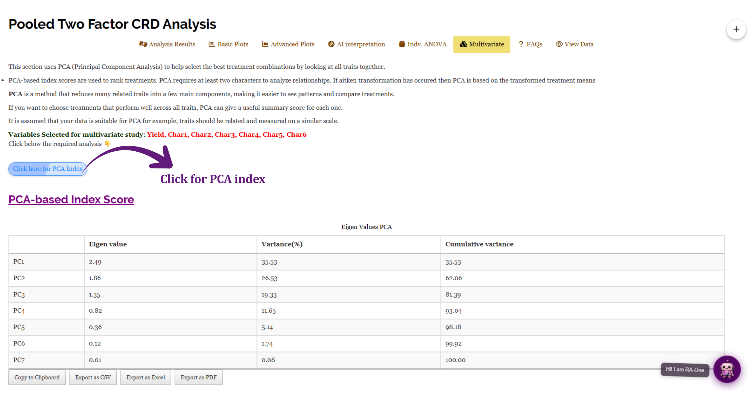
Table 3: PCA eigenvalues for the seven characters
| Component | Eigen value | Variance (%) | Cumulative variance |
|---|---|---|---|
| PC1 | 2.49 | 35.53 | 35.53 |
| PC2 | 1.86 | 26.53 | 62.06 |
| PC3 | 1.35 | 19.33 | 81.39 |
| PC4 | 0.82 | 11.65 | 93.04 |
| PC5 | 0.36 | 5.14 | 98.18 |
| PC6 | 0.12 | 1.74 | 99.92 |
| PC7 | 0.01 | 0.08 | 100.00 |
16.1 Interpretation from Table 3
Seven characters go in, so seven components come out, and the eigenvalues tell you how much of the total variation each one carries. PC1 accounts for 35.53% of the variation and PC2 a further 26.53%, so the first two components together capture 62.06%. Adding PC3 brings the cumulative figure to 81.39%, meaning three components summarise four fifths of everything the seven characters were measuring. The tail is genuinely small: PC6 and PC7 together carry under 2%.
A useful rule of thumb is to keep components with an eigenvalue above 1, since a component carrying less variance than a single standardised character is not summarising anything. By that rule three components matter here (2.49, 1.86 and 1.35), and PC4 onwards (0.82 and below) can be set aside.
Note what a fairly even spread across three components implies: the seven characters are not all measuring the same underlying thing. Had they been strongly correlated, PC1 alone would have absorbed 70% or 80% and the rest would have collapsed. At 35.53% it is doing real work but not dominating, so the index score is a genuine compromise across several distinct dimensions rather than a restatement of one character. Read it alongside the per-character tables, never instead of them.
Use the PCA index for selection across multiple characters, when you must pick one treatment combination and every character matters. It requires at least two characters, since its whole purpose is to exploit the relationships between them, and where an Aitken transformation was applied the PCA is built on the transformed means. It assumes your characters are related and measured on comparable scales. If your characters are genuinely unrelated, as the fairly flat eigenvalue profile above hints, an index will hide more than it reveals, and you are better off reporting each character separately. The eigenvalue table is there so you can make that judgement rather than guess.
Every table on this tab carries Copy to Clipboard, Export as CSV, Export as Excel and Export as PDF buttons beneath it, so the eigenvalues and index scores can go straight into a manuscript without retyping.
17 AI interpretation
You do not have to translate seven ANOVA tables and seven sets of means into prose yourself. The AI interpretation tab turns the whole pooled analysis into a clear, publication-ready narrative (Figure 15). Tick the confirmation box, “I’m not a robot and I have checked that on running analysis there was no error reported”, then click Click here for interpretation. The text streams into a panel with Copy and Stop buttons at the top, so you can lift a defensible paragraph straight into a thesis or report.
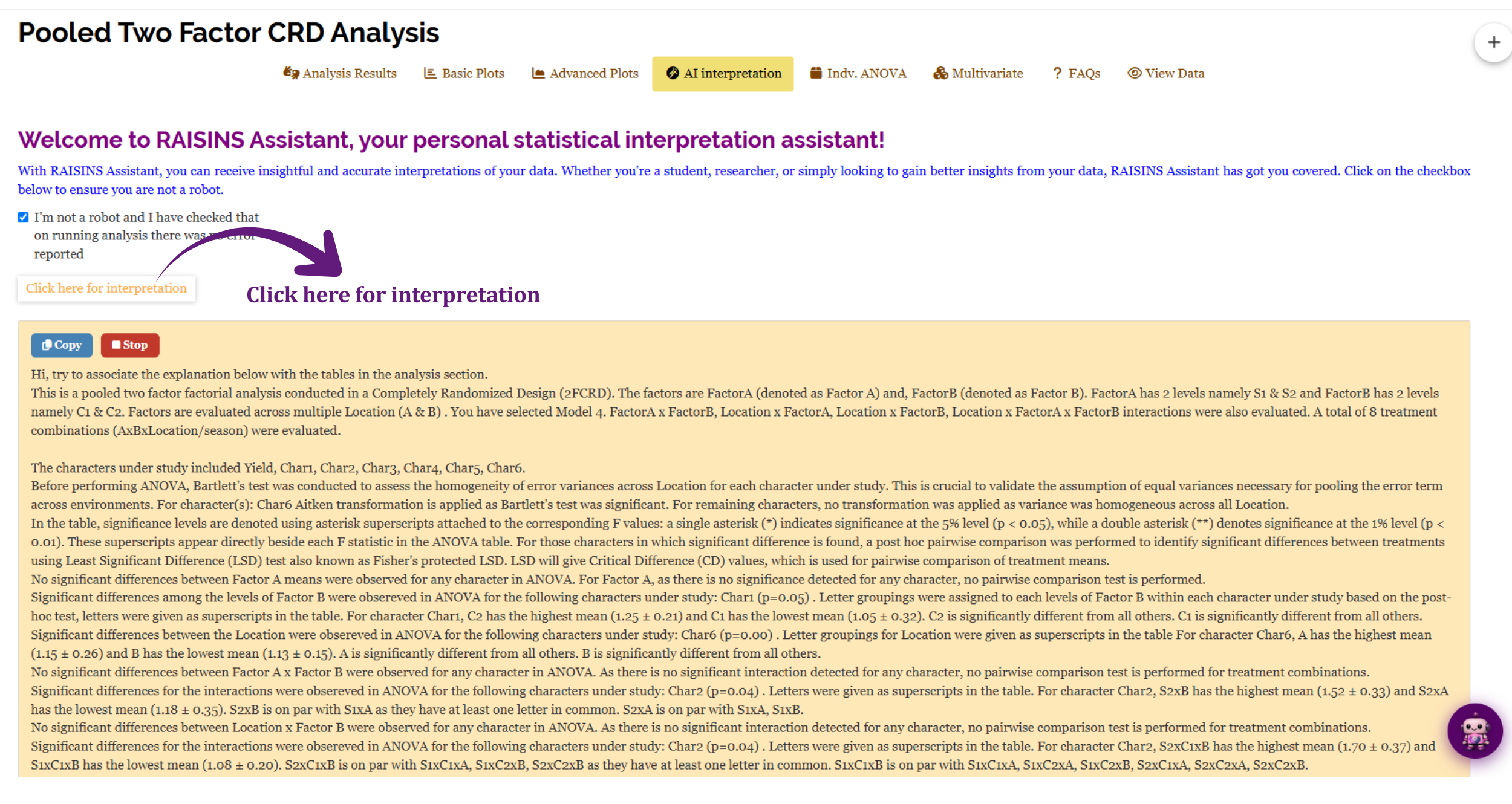
The narrative is not generic boilerplate, it walks the same ladder you walked in Section 2. It opens by restating the design and the model you chose, names the characters under study, and then reports the Bartlett outcome, telling you exactly which characters were Aitken-transformed and which were left alone. It explains the asterisk notation, then works through the sources one at a time: Factor A, Factor B, Location, A × B, and each of the three interactions with Location. For every source it either states that nothing was significant, and therefore no post-hoc test was performed, or it names the significant characters with their p-values and reports the highest and lowest means with their standard deviations and which levels are on par with which.
Read it as a companion to the tables rather than a replacement for them. Its opening line says as much: “Hi, try to associate the explanation below with the tables in the analysis section.”
If the interpretation describes a design that is not the one you ran, the wrong number of levels, the wrong number of locations, the wrong count of treatment combinations, stop and go back to the column selectors on the Analysis Results tab. Because the narrative restates the structure in plain words, it is often the fastest place to catch a column that was assigned to the wrong role.
18 Chat with your data using RA-One
RA-One is the built-in conversational assistant for the Pooled 2FCRD module, reached from the RA-One tab in the green bar or from the floating chat button in the bottom-right corner of any results screen. You ask questions in plain language and it answers using your own analysis rather than generic statistical advice. Every result it discusses is drawn from what the module actually computed, it never invents numbers, and if a value isn’t available it says so instead of guessing. All answers are in plain English, with no code or software commands.
RA-One works directly with your pooled ANOVA, Bartlett test, the means and letter groupings for all seven sources, the PCA index, and the AI interpretation output. In a design with this many interaction terms that is genuinely useful: you can ask it which characters showed a significant Location × Factor A interaction and what that means for your recommendation, why Char6 was Aitken-transformed when the others were not, whether a particular combination is on par with another, or what a critical difference is and why one column is blank. It will explain the general concept and then apply it to your numbers, so you build understanding alongside your results.
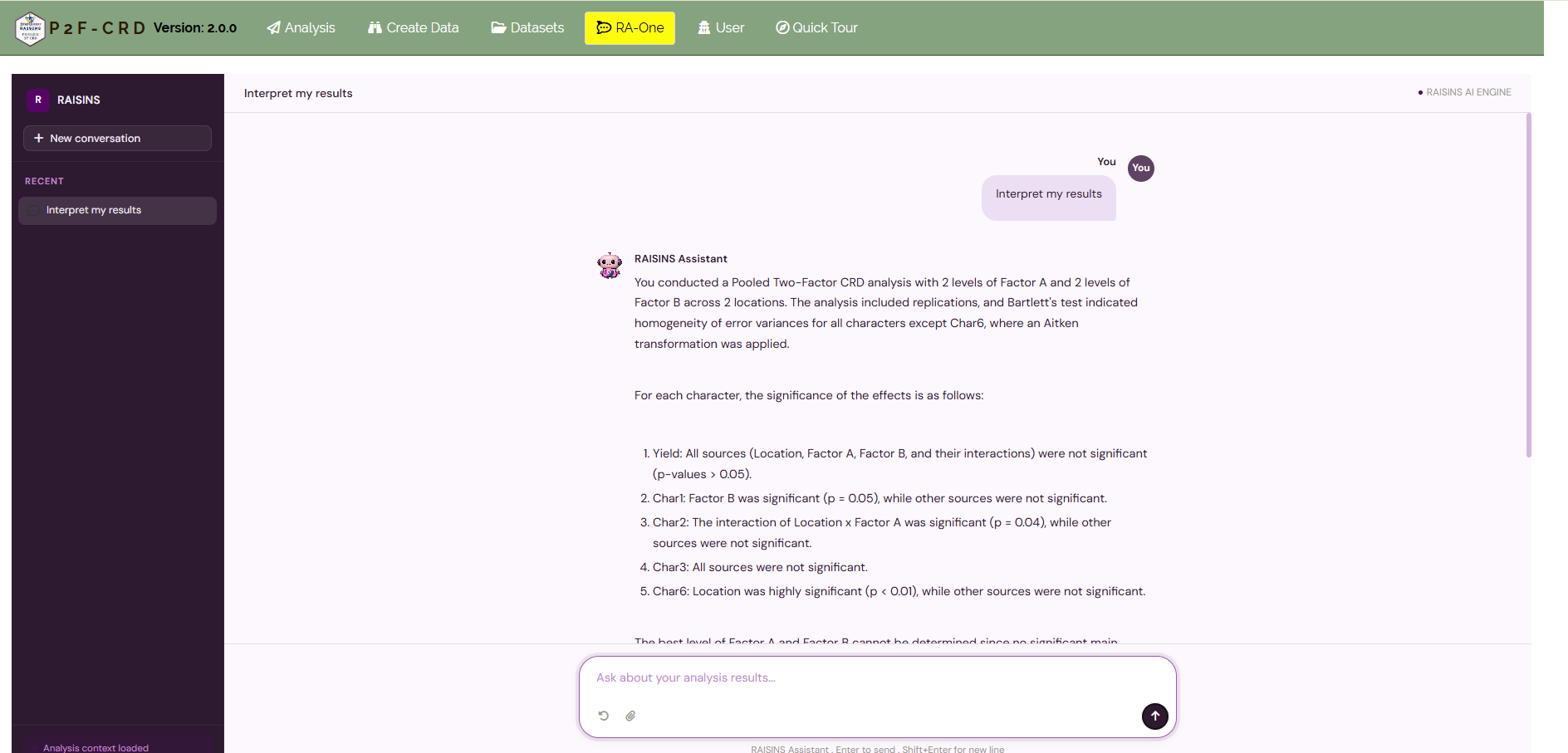
The same chat window can also prepare your data. It can build a correctly formatted pooled 2FCRD dataset template (Section 8.4) for you to fill in, or fetch a model dataset (Section 8.3) so you can try the module straight away, so you never need to leave the tab to get a file ready. RA-One can also generate plots on request, such as an interaction plot for a particular character or a bar chart of combination means, and render them directly in the chat, where you can refine them by asking for changes.
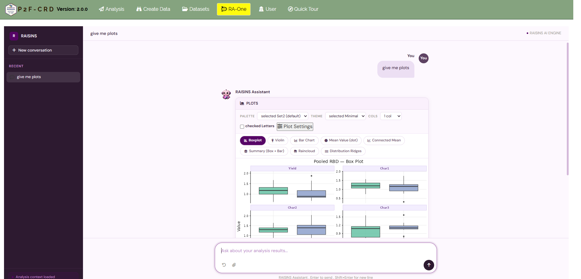
Within a single conversation, RA-One can interpret your pooled results, build a data template, fetch a model dataset, and produce plots, so most of a routine pooled 2FCRD session can be conducted without ever leaving the chat window.
19 FAQs
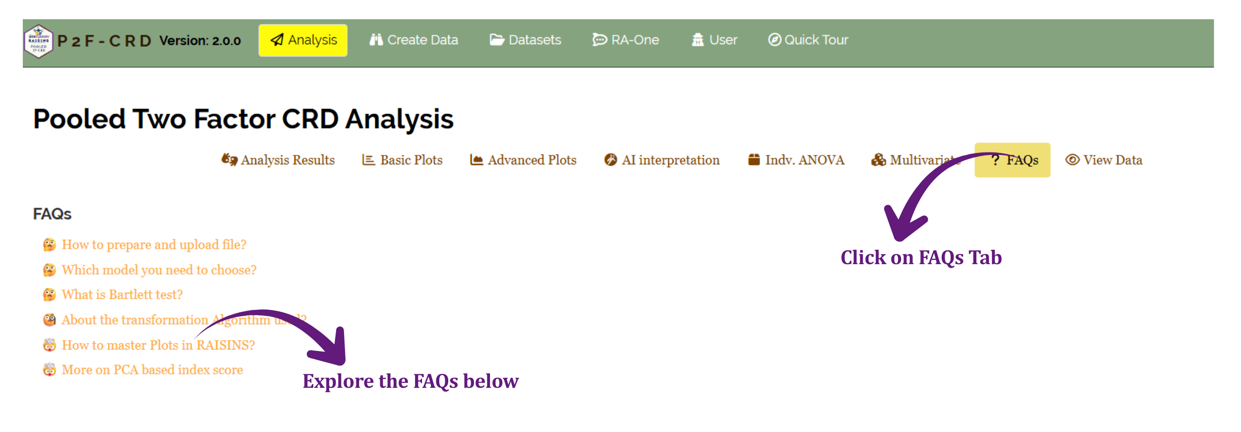
The module includes a dedicated FAQs tab to clarify common doubts and guide you through the features (Figure 18). Six explainers are offered, and they map almost exactly onto the decisions this tutorial asked you to make: How to prepare and upload file?, Which model you need to choose?, What is Bartlett test?, About the transformation Algorithm used?, How to master Plots in RAISINS?, and More on PCA based index score. If you are ever unsure how something works, say why a critical difference column came out blank, or which of the four models fits your sampling scheme, the FAQs are a good place to start.
20 View data
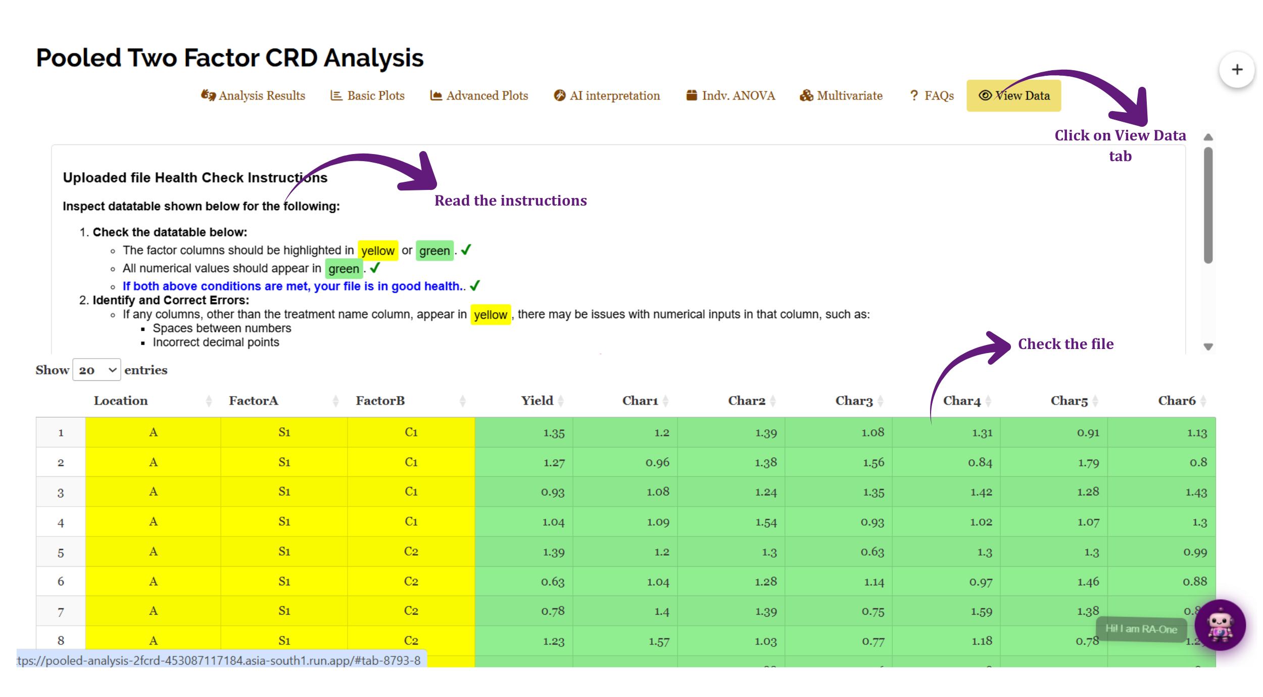
View Data is the primary diagnostic tool for ensuring data integrity before analysis. When you upload your dataset the system performs an automated Health Check, and the tab explains how to read it. The rule is simple and visual: your three factor columns (Location, Factor A, Factor B) should be highlighted in yellow, and every response column should be green. If both conditions are met, the file is in good health.
The colours are also the diagnosis when something is wrong. A column that should hold numbers but appears in yellow is being read as text, which usually means a stray space between digits, an incorrect decimal point, or a non-numeric character hiding in one cell. For a pooled two factor CRD this check is especially worth the ten seconds it takes: it confirms that the environment and both factor columns are being read as categories, that every response column is numeric, and that the factorial is complete, every level of Factor A appearing with every level of Factor B in every environment. A single mistyped label such as “s1” in a column of “S1” silently creates a third factor level and quietly wrecks the pooling.
21 Wrapping up
A pooled two factor CRD rests on one honest question, asked twice over. First: do my two factors act independently, or does the effect of one depend on the other? Second, and more demanding: do either of those answers survive a change of location or season? Everything else, Bartlett’s test, the Aitken transformation, the seven-row ANOVA, the letter groupings, the interaction plots, exists to answer those two questions fairly. RAISINS automates the machinery, from checking that the experiments may be pooled at all to producing the ANOVA and the recommendation, so you can concentrate on what the answer means for your research.
Two habits will serve you well here. Read the interaction rows before the main effects, always, because a significant main effect underneath a significant interaction is close to meaningless. And keep an eye on which characters were transformed, since Aitken-corrected results are stated on a different scale and should be reported as such.
If your design does not match a pooled two factor CRD, the companion modules are there: the CRD and RBD modules for single-environment trials, the Two Factor CRD module when your factorial ran at just one site, and the Pooled CRD and Pooled RBD modules when each environment carried only one treatment factor. And if you get stuck at any point, RA-One is available 24 × 7, or write to us at [email protected].
