Pooled Analysis in RBD
A pooled RBD analysis brings together several randomized block experiments run over different locations or seasons, controlling for blocking within each site, so a treatment can be judged across the whole target region. Read more …
Pooled analysis in a Randomized Block Design (RBD) combines several block-designed experiments conducted across different locations or seasons into a single analysis. Because each experiment uses blocking to control local variation, the pooled analysis accounts for blocks within every environment while it tests whether treatments differ, whether environments differ, and whether the treatment ranking stays the same from one environment to the next. In RAISINS this entire workflow is performed without writing any code. This tutorial walks you through both the statistics and the app, screen by screen.
1 What is a pooled RBD analysis?
Suppose you are evaluating three mango varieties, Alphonso, Kesar, and Dasheri. Testing them at a single orchard would tell you which variety won there, in that one soil, that one season. But a recommendation that only holds at one site is nearly useless: a farmer three districts away wants to know whether the winning variety will still win on their land. So you repeat the experiment at three different locations (Loc1, Loc2, Loc3).
At each location you do not scatter the varieties at random across the whole orchard, because orchards are never uniform, one corner drains better, another gets more shade. Instead you divide each location into blocks (replications), and within every block you grow all three varieties. This is the Randomized Block Design (RBD): blocking soaks up the local variation within a site so that the comparison between varieties is fairer and more precise.
Now you have three separate block-designed results and a genuine question: how do you combine them into one honest conclusion?
Piling all the data into one analysis is the wrong thing to do, because it ignores three facts a multi-location block trial is designed to reveal:
- The blocks within each location differ, and that within-site variation should be removed, not left in the error.
- The locations themselves differ, and that between-site variation should be measured and set aside.
- A variety might win at one location and lose at another. If that happens, no single recommendation is safe, and you need to know it.
A pooled RBD analysis combines the experiments correctly, accounting for blocks within each environment and separating the variation into differences between treatments, differences between environments, and their interaction, then testing each one.
A pooled RBD analysis merges several block-designed repetitions of the same experiment, run across different locations or seasons, into one test that removes block variation within each site and asks whether the treatments differ, whether the environments differ, and whether a treatment’s advantage holds up everywhere.
2 One RBD, or many?
The word that makes a pooled analysis different from an ordinary RBD is environment. An environment is one complete run of your block experiment, one location, or one season, and pooling is the act of combining several of them. Four quantities are in play:
- Block effect - variation between the blocks (replications) within a location. The RBD removes this so it does not muddy the treatment comparison.
- Treatment effect - the difference between your treatments (here, the three mango varieties), averaged over all environments. This is usually what you care about most.
- Environment effect - the difference between the locations or seasons themselves, averaged over all treatments. Real, but usually background.
- Treatment × Environment interaction - whether the treatment differences change from one environment to the next. This is the quantity that a single-location trial can never measure, and the reason multi-location testing exists.
If the interaction is not significant, every environment tells the same story, the best treatment is best everywhere, and you may quote one overall recommendation with confidence. If the interaction is significant, the treatments rank differently in different environments (a “crossover”), and quoting a single winner would be misleading, you must instead say which treatment wins where. Checking the interaction is the single most important step in reading a pooled analysis.
This is why you cannot simply stack the data and run one analysis: doing so throws the block, environment, and interaction effects into the error term, inflating it and hiding the very effects you set out to study. The pooled RBD analysis keeps them separate.
3 How RAISINS runs a pooled RBD
There is a fixed order of operations behind a pooled analysis, and RAISINS follows it for you. The logic goes like this:
- Analyse each environment on its own as a simple RBD (accounting for its blocks), and record its error variance.
- Ask whether those error variances are equal across environments, using Bartlett’s test. This is the gatekeeper: you are only allowed to pool experiments whose noise is comparable.
- If the variances are homogeneous, pool the data directly. If they are heterogeneous, re-scale each environment first, using the Aitken transformation, so that every environment carries equal weight.
- Build the pooled ANOVA, partitioning variation into Treatment, Environment, the block-within-environment effect, and the Treatment × Environment interaction.
- Read the interaction first, then interpret treatment and environment means with the appropriate multiple-comparison test.
Figure 1 shows this as a single picture.
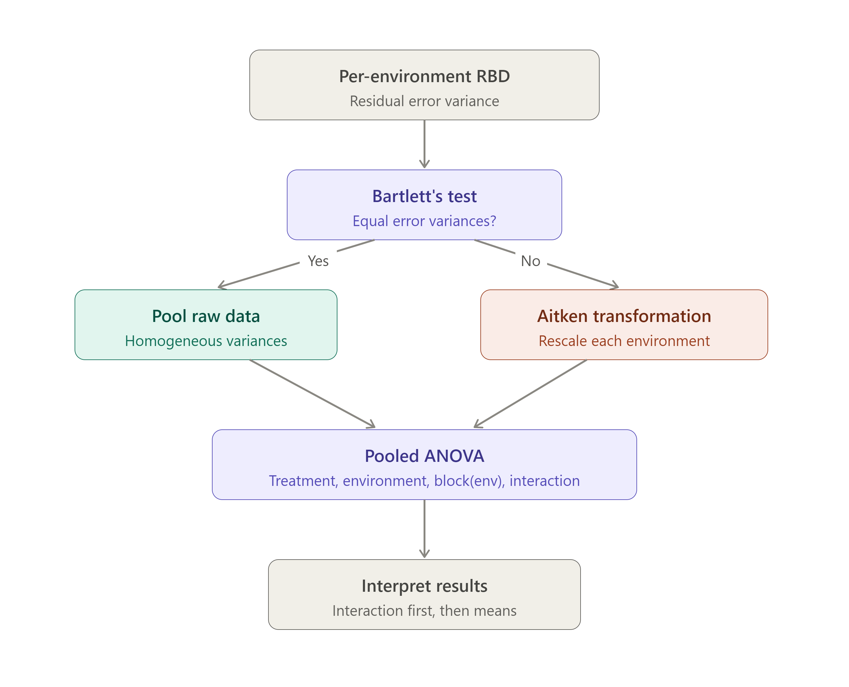
RAISINS runs the individual analyses, performs Bartlett’s test, applies the Aitken transformation only where it is needed, assembles the pooled ANOVA under the model you choose, and attaches letter groupings, all from a single click of Run Analysis. The flowchart is here so you understand why the software did what it did, not because you must do it yourself.
4 Assumptions of a pooled RBD
A pooled RBD analysis inherits the assumptions of the ordinary RBD and adds one of its own, homogeneity of error variance across environments.
| Assumption | What it means | What if it fails? |
|---|---|---|
| Complete blocks | Every treatment appears once in every block, at every location | Serious. Settled by design; an incomplete-block design needs a different module |
| Randomisation | Within each block, treatments are assigned to units at random | Settled by good design, not fixable at the analysis stage |
| Additivity | Block and treatment effects add up, with no block × treatment interaction within a site | If blocks and treatments interact, consider a transformation |
| Normality | Errors within each environment are approximately normal | Try a log, square-root, or arcsine transformation (Section 11) |
| Homogeneity of variance across environments | Each environment’s error variance is roughly the same | RAISINS checks this with Bartlett’s test and applies the Aitken transformation automatically when it fails (Section 12) |
| Continuous response | The measurement is a proper number (yield, sugar), not a category | Use a method designed for that data type instead |
The one assumption unique to pooling, equal error variance across environments, is the one you do not have to police yourself. RAISINS tests it for every trait and repairs it where needed, before it builds the pooled ANOVA. Your job is to design each environment’s block experiment well and randomise properly; RAISINS handles the rest.
5 Getting to the module
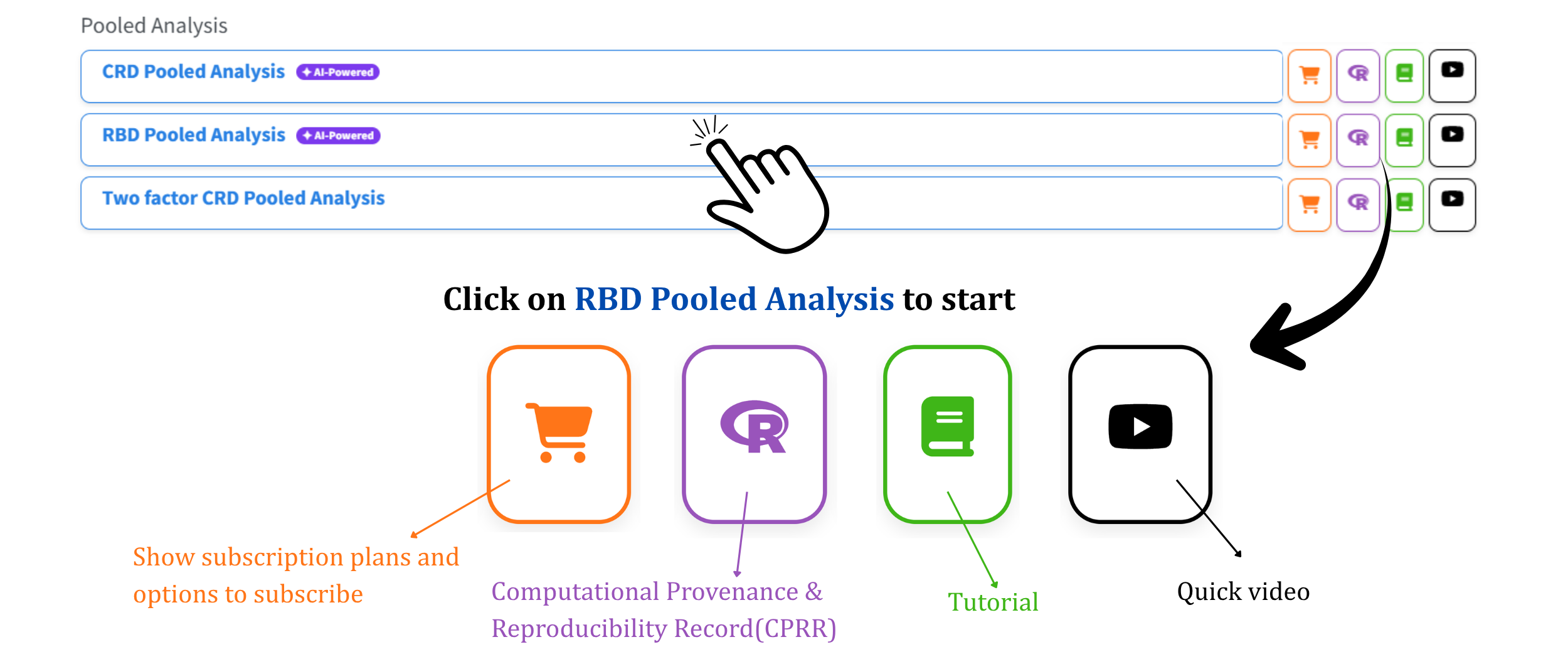
Now that the theory is clear, let us run the analysis. Visit the RAISINS home page at www.raisins.live and go to Data Analysis. Under Pooled Analysis, click RBD Pooled Analysis to start, as shown in Figure 2.
5.1 Computational Provenance & Reproducibility Record
CPRR (Computational Provenance & Reproducibility Record) provides a transparent and comprehensive record. Click the CPRR icon shown in Figure 2 to access it and know about the computational workflow performed during the analysis. The record for this module states the R version and the exact version of every package used, and names the specific function behind each reported result. CPRR lists every default parameter and decision rule applied by the module and provides fully runnable R code that reproduces each analytical step. Users can execute the code in R to independently reproduce and verify the results. It carries its own DOI.
To cite the platform itself in a paper, thesis, or report, use the RAISINS citation, available in APA, Harvard, and BibTeX formats at www.raisins.live/citation.html. That is the primary reference, and for most manuscripts it is all you need.
The CPRR for the Pooled Analysis in RBD module is at www.raisins.live/module_record/pooledrbd.html.
Cite the RAISINS paper as your primary reference for the platform. Add the CPRR as supporting documentation when a journal asks for details of the computing environment, or when you want your methods section to be precise about versions and functions rather than saying “analysis was carried out using an online tool.” The CPRR supports the citation and ensures computational reproducibility.
6 Preview mode and Quick Tour
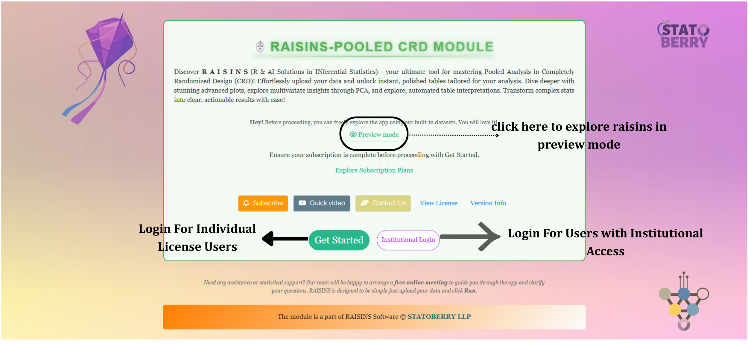
Before subscribing, you can explore the entire module using Preview mode, reached from the welcome page shown in Figure 3 by clicking the Preview mode link. Preview mode loads built-in datasets so you can try every feature (the pooled ANOVA, Bartlett test, plots, individual analyses, the multivariate index, and the RA-One assistant) without uploading your own data. The same page offers Get Started for individual-licence users and Institutional Login for institutional access. First-time users are also offered a Quick Tour, an interactive, step-by-step walkthrough that highlights each control and explains what it does. You can retake the tour at any time from the Quick Tour tab.
7 A working example
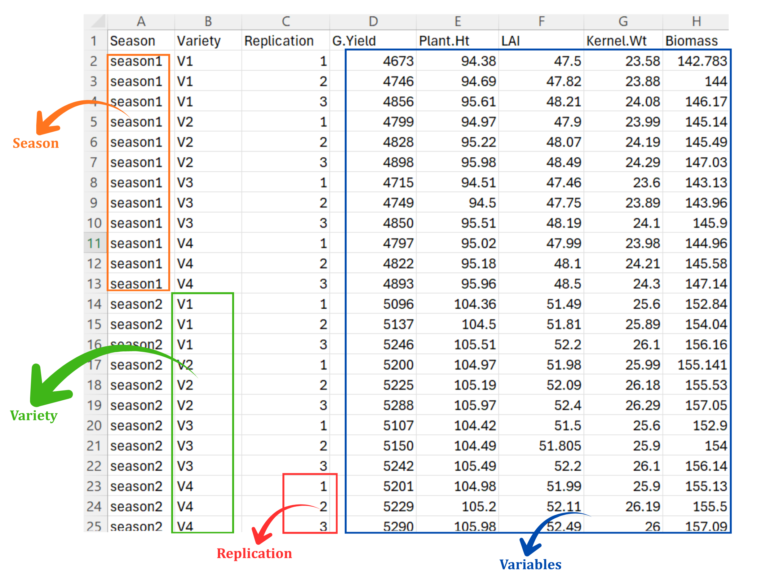
This tutorial uses a mango variety trial. Three varieties, Alphonso, Kesar, and Dasheri, were grown as a randomized block design at three locations (Loc1, Loc2, Loc3), with three blocks (replications) per location. For every plot, two response variables were recorded, Yield and Sugar content, illustrating how RAISINS analyses several traits in a single run (Figure 4). Each trait is pooled across the three locations independently, producing its own set of results. The task is to determine which variety performs best, whether the locations differ, whether the blocking was worthwhile, and, most importantly, whether the best variety is the same at every location.
8 How to prepare your data
Your analysis is only as good as your data. Feed RAISINS high-quality data and it will deliver powerful insights; feed it messy data and the results will not be trustworthy. You have four routes:
- Create your dataset in MS Excel
- Build your dataset directly within the RAISINS app
- Using the Model datasets in RAISINS as a reference
- Create your dataset using the RA-One chat assistant
8.1 Preparing data in MS Excel
Open a new blank sheet in MS Excel containing only one sheet, and avoid adding any unnecessary content. The dataset should follow a column-based format with a clear structure for pooled RBD:
- The first column holds the environment label, the location or season (e.g. “Loc1”, “Loc2”, “Loc3”).
- The treatment column holds the treatment label (e.g. “Alphonso”, “Kesar”, “Dasheri”).
- The block column holds the block or replication number within each location (e.g. 1, 2, 3).
- Every response variable under study (e.g. Yield, Sugar) occupies its own separate column.
Each environment label repeats for every observation recorded in it, and within each environment each treatment appears once in every block. The file can be saved as CSV, XLS, or XLSX, but CSV is recommended as it is lighter and loads faster. Ensure there are no unwanted spaces in the column names or in the labels. For reference, see the structure in Figure 4.
Dataset creation rules
- Column naming convention
- No spaces allowed in column names.
- Use underscores (
_) or full stops (.) for separation. - Avoid symbols and special characters such as %, #.
- Data arrangement
- Start the data towards the upper-left corner.
- Ensure the row above the data is not blank.
- Keep the environment, treatment, and block columns clearly labelled.
- Cell management
- Avoid typing or deleting in cells without data.
- If needed, select the affected cells, right-click, and choose Clear Contents.
- Balance and completeness
- Every treatment should appear once in every block, in every environment.
- Keep the number of blocks consistent across locations so the design stays balanced.
- Labels
- Keep the spelling and capitalisation of environment, treatment, and block labels perfectly consistent, “Loc1” and “loc1” would be read as two different locations.
How to save as CSV in MS Excel
Open your workbook. Ensure your data is arranged properly with only one sheet.
Click the ‘File’ menu. Go to the top-left corner and click File.
Choose ‘Save As’ or ‘Save a Copy’. Select the location where you want to save your file.
Set file type to CSV. In the ‘Save as type’ dropdown, choose CSV (Comma delimited) (*.csv).
Name your file. Enter a relevant file name without spaces (use underscores if needed).
Click ‘Save’. Click Save to export the file.
💡 Tip: Before saving, double-check that your data is on the first sheet and follows the required format: no empty rows above the data, meaningful column names, and an environment, treatment, and block column plus one column per response variable.
8.2 Prepare using Create Data in RAISINS
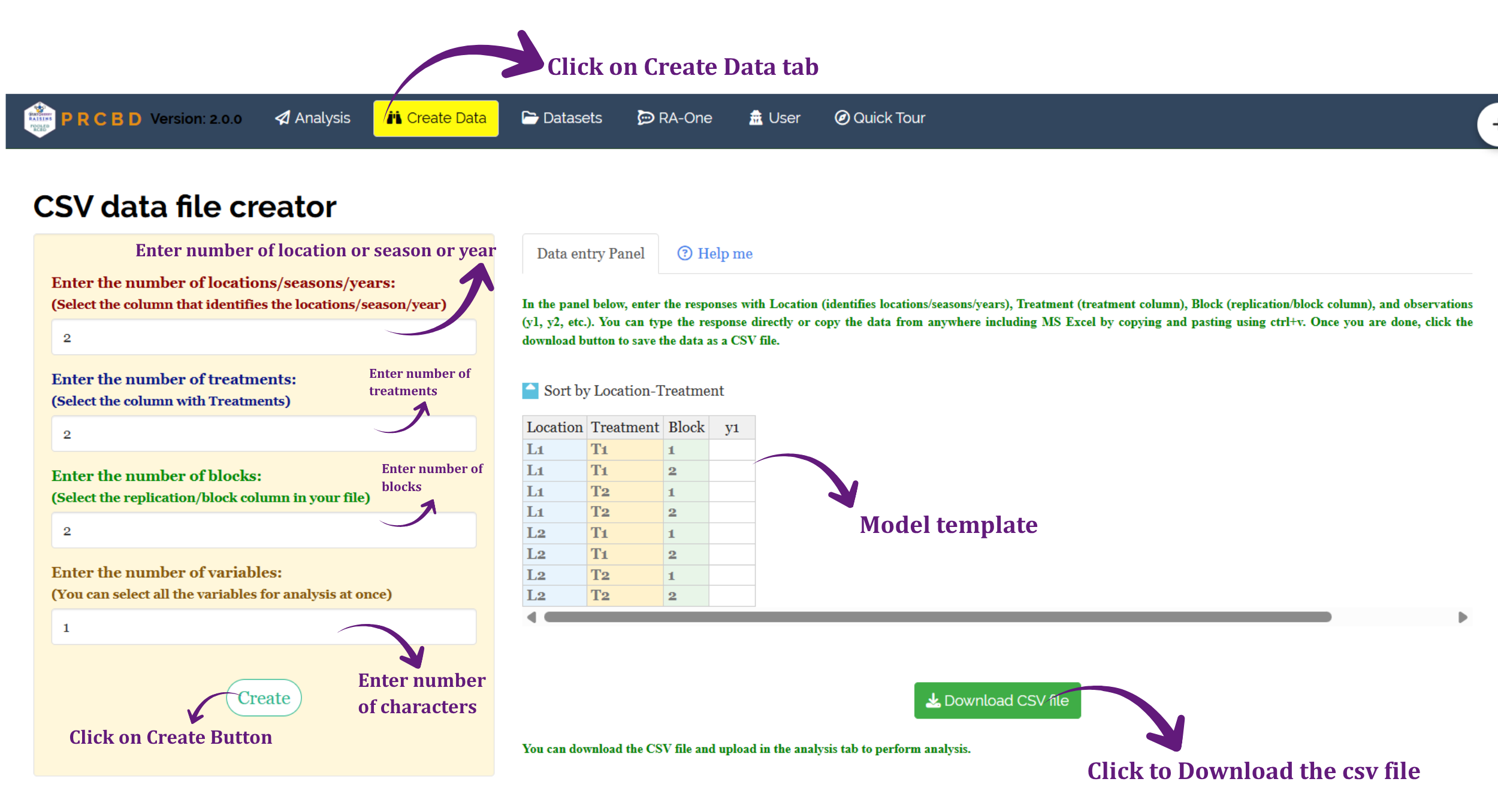
If you are unsure about the correct format, do not worry, RAISINS can create the data layout for you using the prescribed template. Here is how:
- Navigate to the Create Data tab
- Select the number of Locations / Seasons (environments)
- Select the number of Treatments
- Select the number of Blocks (Replications)
- Select the number of Variables
- Click the Create button
The model layout appears as shown in Figure 5, with the environment, treatment, and block columns already laid out. You may enter the observations manually into the CSV once downloaded, or paste them straight into the file provided. Once the observations are entered, download the CSV and upload it under Analysis Results.
8.3 Download Model Datasets
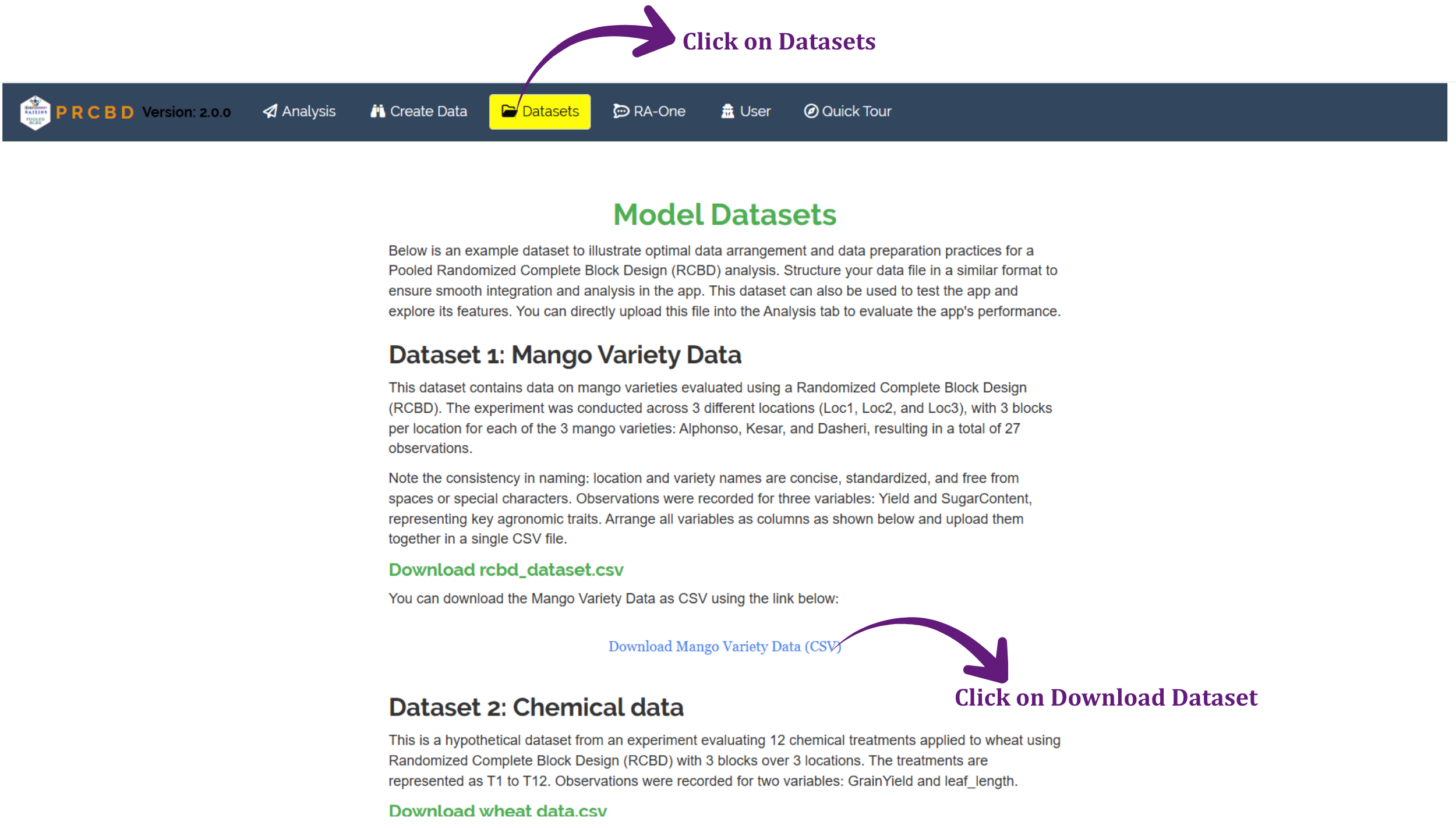
If you are unsure about the required data format or would like to explore the module before using your own data, RAISINS provides model datasets for reference, including the mango dataset used in this tutorial. To download them:
- Navigate to the Datasets tab
- Click the Download CSV link corresponding to the required dataset
- Save the file to your computer
- Use the model dataset as a reference for preparing your own data, or upload it directly to explore the analysis
8.4 Creating a dataset using RA-One chat
RA-One, the built-in chat assistant, can help you create a properly formatted dataset through a simple conversation. To get started, open the RA-One chat by clicking the chat icon available within the app or by heading over to the RA-One tab. You can tell it the number of locations, treatments, blocks, and response variables, and RA-One will generate a dataset in the required pooled-RBD format. You can review the generated dataset in the chat, download it as a CSV file, and upload it directly under the Analysis Results tab. The full workflow is illustrated in Figure 7 below.
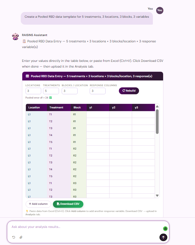
RA-One chat workflow: opening the chat, generating the dataset, and downloading the CSV
9 The Analysis Results tab
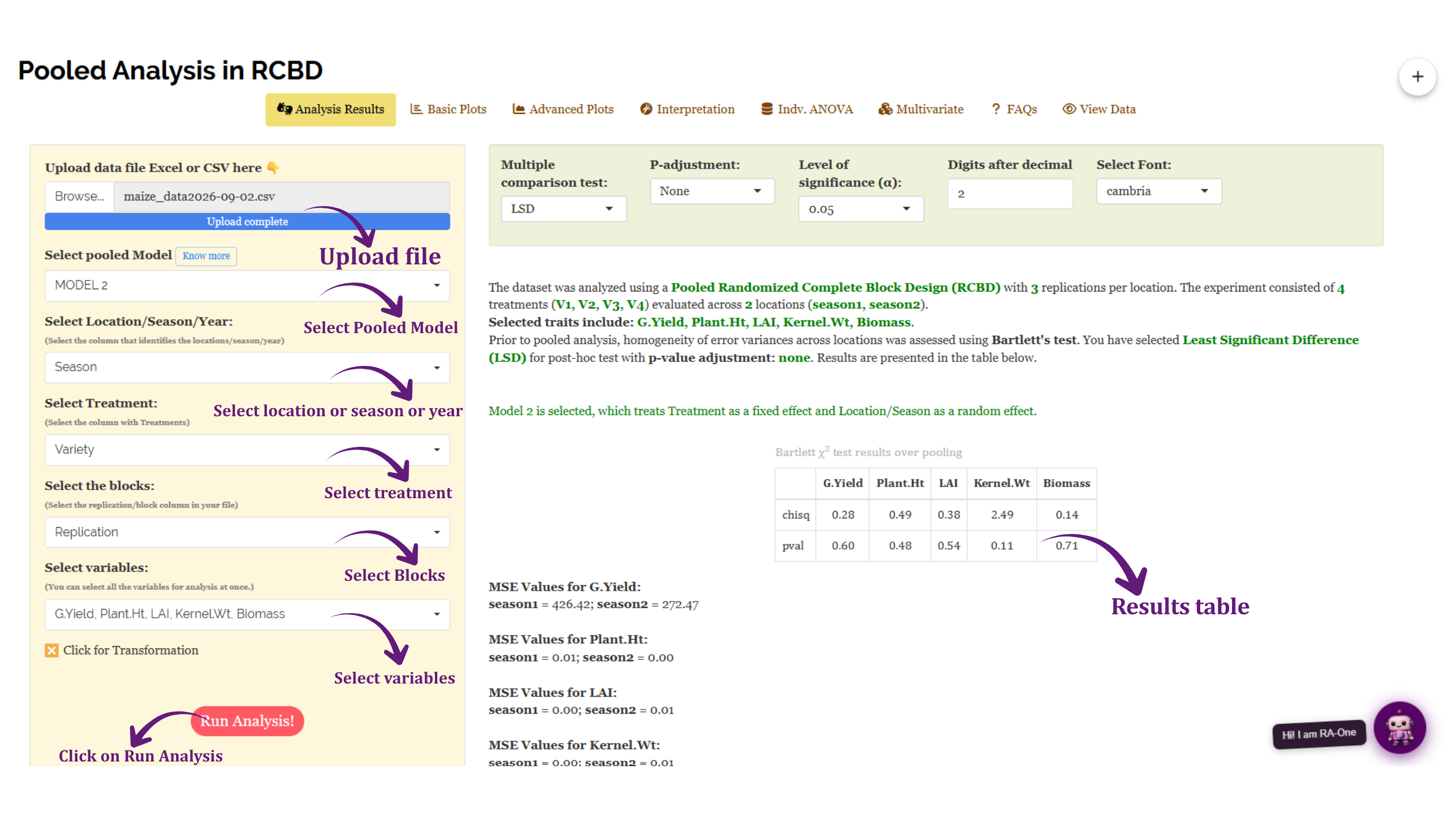
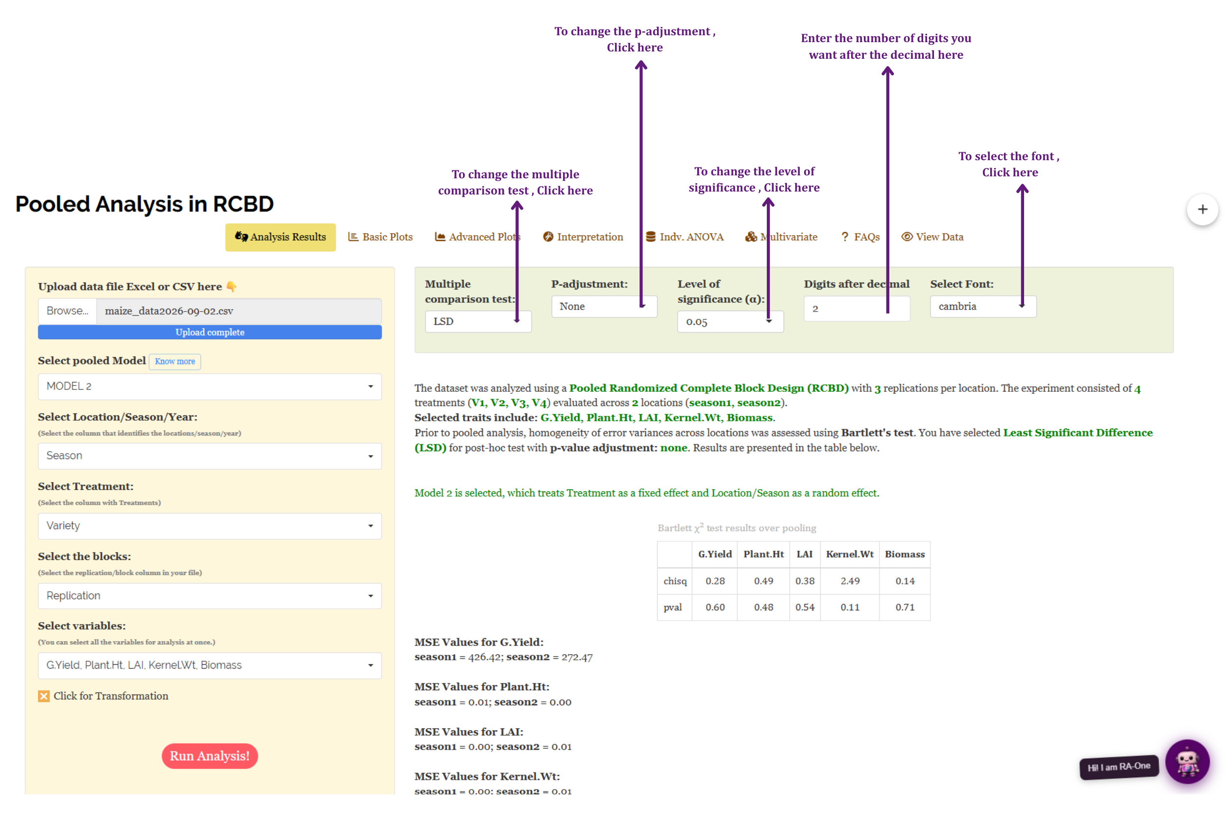
Figure 8 shows the Analysis Results tab in detail. Upload your prepared file by clicking Browse in the sidebar. Once uploaded, selectors appear for the pooled model, the environment column (Location/Season/Year), the treatment column, the block column, and the response variables. Choose each one, then click Run Analysis. All outputs then appear across the sub-tabs: Analysis Results, Basic Plots, Advanced Plots, Interpretation, Indv. ANOVA, Multivariate, FAQs, and View Data.
On the results panel you can adjust the multiple-comparison test (LSD, Tukey’s HSD, or DMRT), the P-adjustment, the significance level (α), the number of decimal digits, and the font. If a trait turns out not to be normally distributed, RAISINS provides a built-in transformation option (Section 11), and if the error variances are unequal across environments it applies the Aitken transformation automatically (Section 12).
Which multiple-comparison test should I pick?
LSD (Least Significant Difference) is the default and the most sensitive, it declares two means different as soon as they differ by more than the critical difference. It is a good general choice for a well-designed trial.
Tukey’s HSD (Honestly Significant Difference) is more conservative and controls the error rate across all pairwise comparisons at once, a safer choice when you have many treatments and want to guard against false positives.
DMRT (Duncan’s Multiple Range Test) sits between the two and is traditional in agricultural research.
All three produce the same kind of letter grouping; they differ only in how strict the cut-off is. When in doubt, LSD is a reasonable default, and RAISINS lets you switch and re-read instantly.
10 Choosing a pooled model
Before it reports a single number, the module asks one structural question: are your treatments and your environments fixed things you chose deliberately, or a random sample of a larger population? The answer changes which error term each effect is tested against, and RAISINS lets you state it explicitly through the Select pooled Model control. There are four choices:
| Model | Treatment | Location / Season | Read it as |
|---|---|---|---|
| Model 1 | random | random | Both the treatments and the environments are samples of larger sets |
| Model 2 | fixed | random | You care about these specific treatments, tested across a random sample of environments |
| Model 3 | random | fixed | You care about these specific environments, testing a random sample of treatments |
| Model 4 | fixed | fixed | Both the treatments and the environments are the only ones you care about |
In the mango working example we selected Model 2, which treats Treatment as a fixed effect and Location/Season as a random effect. This is the most common choice in variety and treatment trials: you have three specific mango varieties you want to compare (fixed), and the three locations stand in for the wider growing region you hope to generalise to (random). RAISINS states your selection in plain language at the top of the results (Figure 9) so there is never any doubt about which model produced the numbers below.
Under a fixed-effects model an effect is tested against the pooled error. Under a mixed model like Model 2, a random environment changes the correct denominator for the F-test of the main effects, most importantly, it means the Location × Treatment interaction becomes the natural yardstick for judging whether a treatment difference holds up across environments. You do not have to work any of this out yourself: once you pick the model, RAISINS assembles the correct F-tests automatically.
11 Transformation
Two distinct kinds of transformation live in this module, and it helps to keep them apart.
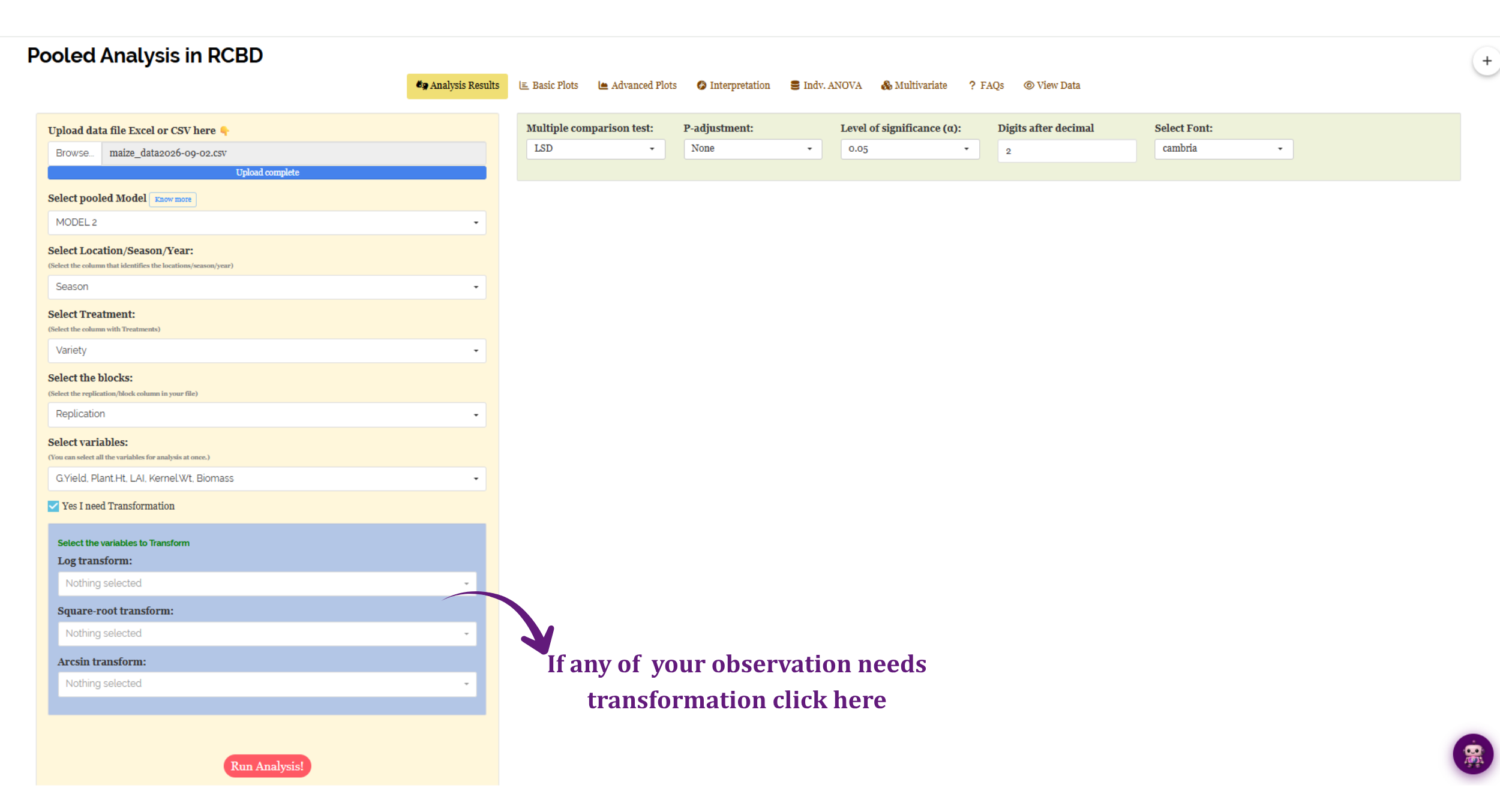
The Aitken transformation is applied automatically and only when Bartlett’s test finds the error variances unequal across environments (Section 12). You do not choose it; RAISINS applies it for you where the data demand it.
The normalising transformations, logarithmic, square-root, and arcsine, are ones you apply manually when a trait is not normally distributed. Switch on the transformation option in the sidebar and select the variables to transform, as shown in Figure 10.
Logarithmic transformation converts a skewed distribution into a more symmetrical one by replacing each data point (x) with its logarithm. It is applied to positive, continuous data where the variance grows in proportion to the mean, a pattern common in phenomena that grow multiplicatively.
Square root transformation stabilises variance and reduces right-skewness by replacing each data point (x) with its square root. It is primarily used for non-negative count data, such as those following a Poisson distribution, where variance increases with the mean.
Arcsine transformation (the angular transformation) is designed for proportions or percentages bounded between 0 and 1. By taking the inverse sine of the square root of the proportion, it stretches the ends of the distribution near 0 and 1, where variance is naturally small.
After choosing any transformation, proceed to Section 12 and Section 13 for the analysis.
12 Homogeneity of variance and the Aitken transformation
The whole point of a pooled analysis is to combine several experiments into one. But you are only allowed to pool them if the experiments are measuring on comparable terms, specifically, if the error variance is roughly the same in every environment. If one location is wildly noisier than the others, throwing all the data into a single error term would let that one messy location contaminate every comparison. So before pooling, RAISINS checks this with Bartlett’s test, applied to each response variable across the locations.
Bartlett’s test takes the error variance (the MSE) from each location’s individual RBD and asks whether they are all equal. Its null hypothesis is that the variances are homogeneous. A large p-value (≥ 0.05) is the “good” outcome here, it means the variances are compatible and the experiments may be pooled directly. A small p-value (< 0.05) means at least one location wobbles by a different amount, and the data must be re-scaled before pooling.
Table 1: Bartlett χ² test for homogeneity of error variances across locations
| Statistic | Yield | Sugar |
|---|---|---|
| χ² | 0.00 | 0.27 |
| p-value | 1.00 | 0.88 |
Table 1 reports Bartlett’s chi-square statistic and its p-value for both traits in the mango example. Both p-values are comfortably above 0.05, so the error variances are homogeneous across the three locations for both traits. You can see why in the per-location MSE values printed beneath the table on screen: for Yield the error variance is identical everywhere (Loc1 = 0.15, Loc2 = 0.15, Loc3 = 0.15), and for Sugar it is close (0.07, 0.11, 0.11). Because neither trait failed the test, RAISINS prints the message “No Aitken transformation applied. Variance is homogeneous for all characters across all Location,” and proceeds to pool the raw data as they are.
Had a trait failed Bartlett’s test, RAISINS would automatically apply the Aitken transformation to that trait, dividing each location’s observations by the square root of that location’s MSE, which puts every environment on an equal-variance footing before pooling. The transformed values would then carry through the ANOVA, and the transformed means would appear in parentheses in the results tables. This happens silently and only for the offending traits; the others are left untouched. You never lose the ability to pool, RAISINS simply repairs the scale first.
13 The pooled ANOVA
With the homogeneity check passed, RAISINS builds the pooled analysis of variance. This is the heart of the module. Instead of three separate RBD tables, one per location, you get a single table that partitions the total variation into interpretable sources plus error, and tests each one. Compared with a pooled CRD, the RBD table carries one extra row, Location × Block, which captures the block (replication) variation within each environment.
Table 2: Pooled ANOVA - mean squares and significance
| Source of variation | DF | Yield | Sugar |
|---|---|---|---|
| Location | 2 | 2.25** | 5.38** |
| Treatment | 2 | 233.6** | 951.73** |
| Location × Block | 6 | 0.04 NS | 0.57** |
| Location × Treatment | 4 | 0 NS | 0.08 NS |
| Pooled Error | 12 | 0.15 | 0.10 |
Each cell is a mean square, and the asterisks encode significance: ** marks the 1% level, * the 5% level, and NS means non-significant. Read the table one row at a time, because each row answers a different research question.
13.1 Interpretation from Table 2
Treatment is the row you most likely care about, and it is overwhelmingly significant for both traits (Yield MS = 233.6**, Sugar = 951.73**, each significant at the 1% level). The three mango varieties genuinely differ in yield and sugar, and they do so consistently enough across the three locations to show up in the pooled test.
Location is also significant for both traits (2.25**, 5.38**). This tells you the three environments themselves differ, some sites are simply more productive than others, which is expected and confirms there was real environmental variation to pool over.
Location × Block is the row unique to a pooled RBD, and it reports whether the blocking mattered. It is non-significant for Yield (0.04 NS) but significant for Sugar (0.57**). For Sugar, the blocks captured real local variation within the sites, which means the blocking was worthwhile: an RBD removed noise that a CRD would have left in the error, sharpening the treatment comparison. For Yield, the block effect was negligible, but blocking did no harm.
Location × Treatment is the most important row to read carefully, and here it is non-significant for both traits (0 NS, 0.08 NS). This is the best possible outcome for a plant breeder or agronomist. A non-significant interaction means the ranking of the varieties does not change from location to location, the variety that is best at Loc1 is best at Loc2 and Loc3 too. Because of this, you are entitled to interpret the overall treatment means directly and make a single recommendation that holds across all three locations.
In any multi-environment trial the interaction row is the gatekeeper for your conclusions. If the interaction is significant, the treatments rank differently in different environments, and quoting a single “best treatment overall” would be misleading, you would instead study the Location × Treatment table (Section 16) to see which treatment wins where. If the interaction is non-significant, as it is here, the main-effect means are safe to interpret on their own. Always check this row first, before celebrating a significant Treatment effect.
14 Treatment means and grouping
A significant Treatment row in the ANOVA tells you the varieties differ, but not which differs from which. That is the job of the multiple-comparison test (LSD, Tukey’s HSD, or DMRT, chosen in the sidebar), which attaches letter groupings to the means: treatments sharing a letter are not significantly different, treatments with different letters are. Table 3 shows this for the mango example.
Table 3: Treatment means (mean ± SD with letter grouping) and key statistics
| Variety | Yield | Sugar |
|---|---|---|
| Alphonso | 10.10 ± 0.52 c | 30.01 ± 0.78 c |
| Dasheri | 20.29 ± 0.53 a | 50.57 ± 0.86 a |
| Kesar | 14.95 ± 0.52 b | 40.34 ± 0.78 b |
| F stat | 59335.05** | 11296.74** |
| CD (Treatment) | 0.08 | 0.38 |
| CV (%) | 0.42 | 0.72 |
14.1 Interpretation from Table 3
Every mean carries a different letter (a, b, c) for both traits, which means all three varieties are significantly different from one another, no two share a group. The ordering is identical across traits: Dasheri (a) > Kesar (b) > Alphonso (c). Dasheri is the clear top performer, roughly doubling Alphonso’s yield (20.29 vs 10.10) and carrying the highest sugar (50.57).
The critical difference (CD) is the yardstick for these comparisons: two varieties differ significantly only if their means are further apart than the CD. For Yield the CD is just 0.08, and the varieties are separated by five to ten units, so the differences are overwhelming. The very low CV values (0.42% and 0.72%) confirm this was a highly precise experiment, the within-group noise is tiny relative to the differences between varieties, which is exactly why the F-statistics are so enormous, and part of that precision comes from the blocking.
Because the Location × Treatment interaction was non-significant (Section 13), this single ranking is trustworthy at every location. If your goal is to recommend one variety across the whole region, Dasheri is the answer on both traits.
RAISINS decides the letter groupings using the full-precision CD and prints a rounded CD in the table. Occasionally two means that look closer than the printed CD still receive different letters, because the grouping used more decimal places than the display shows. The letters are always the authoritative statement of significance.
15 Location means and grouping
The same multiple-comparison machinery is applied to the environments, so you can see which locations were more productive. Table 4 presents the result.
Table 4: Location means (mean ± SD with letter grouping) and key statistics
| Location | Yield | Sugar |
|---|---|---|
| Loc1 | 15.10 ± 4.39 b | 39.58 ± 8.88 c |
| Loc2 | 15.62 ± 4.44 a | 40.23 ± 9.01 b |
| Loc3 | 14.62 ± 4.44 c | 41.12 ± 8.87 a |
| F stat | 15.29** | 55.94** |
| CD (Location) | 0.39 | 0.32 |
| CV (%) | 2.54 | 0.77 |
15.1 Interpretation from Table 4
The locations differ significantly for both traits, but note two things. First, the spread of the location means is small compared with the spread of the variety means, Yield ranges only from 14.62 to 15.62 across locations, versus 10.10 to 20.29 across varieties, so environment matters far less than variety here. Second, the standard deviations are large (e.g. 4.39 for Loc1 Yield) precisely because each location average is taken across all three varieties, which themselves differ hugely; that within-location spread is variety signal, not error.
The rankings differ by trait: Loc2 gives the highest Yield (15.62 a) and Loc3 the highest Sugar (41.12 a). This is ordinary environmental variation, some sites favour one trait over another, and it is exactly the kind of background variation the pooled design is built to account for while it isolates the treatment effect you actually care about.
16 The interaction table
Finally, Table 5 reports the mean of every Location × Treatment combination, all nine cells for the mango example. This table is where you would hunt for crossover effects if the interaction had been significant.
Table 5: Location × Treatment combination means (mean ± SD)
| Combination | Yield | Sugar |
|---|---|---|
| Alphonso × Loc1 | 10.12 ± 0.34 | 29.24 ± 0.35 |
| Alphonso × Loc2 | 10.60 ± 0.34 | 29.89 ± 0.34 |
| Alphonso × Loc3 | 9.60 ± 0.34 | 30.89 ± 0.34 |
| Dasheri × Loc1 | 20.23 ± 0.34 | 49.71 ± 0.61 |
| Dasheri × Loc2 | 20.82 ± 0.34 | 50.67 ± 0.34 |
| Dasheri × Loc3 | 19.82 ± 0.34 | 51.34 ± 0.67 |
| Kesar × Loc1 | 14.96 ± 0.33 | 39.78 ± 0.34 |
| Kesar × Loc2 | 15.45 ± 0.33 | 40.12 ± 0.67 |
| Kesar × Loc3 | 14.45 ± 0.33 | 41.12 ± 0.67 |
| F stat | 0.03 NS | 0.88 NS |
| p value | 1.00 | 0.51 |
The interaction F-statistics at the foot of the table are non-significant for both traits (Yield 0.03 NS, Sugar 0.88 NS; p = 1.00, 0.51), which is why the CD (Location × Treatment) row is left blank, when an effect is not significant, RAISINS deliberately suppresses the critical difference so you are not tempted to read into differences that are statistically indistinguishable. The nine combination means are reported for completeness, but you should not compare them with letters.
Reading the cells confirms the story from Section 13: within every location the order is the same, Dasheri > Kesar > Alphonso. For Yield, Dasheri scores 20.23, 20.82, and 19.82 across the three locations while Alphonso scores 10.12, 10.60, and 9.60, the gap between the varieties is enormous and steady, and the varieties never swap places. This visual constancy is precisely what a non-significant interaction looks like in the raw means.
The error variances were homogeneous across locations, so the three block experiments were pooled directly with no Aitken transformation. In the pooled ANOVA, variety and location both mattered; the blocking was worthwhile for Sugar; but the variety × location interaction did not matter, so a single variety recommendation holds everywhere. Dasheri was significantly the best variety for both yield and sugar at all three locations, with Alphonso the poorest and Kesar in between. That is the entire experiment in one sentence, and RAISINS assembled it for you.
A glossary of the result-table rows
Mean ± SD - each cell is the average of that treatment (or location, or combination) followed by its standard deviation. Where an Aitken transformation was applied, the transformed mean is shown in parentheses.
Letter grouping (a, b, c) - attached by the multiple-comparison test. Means sharing a letter are not significantly different at the chosen α; means with different letters are.
F stat - the ratio testing whether that factor’s means differ. The asterisks (* 5%, ** 1%, NS not significant) come straight from this statistic.
Location × Block - the pooled block (replication) effect within environments, unique to the RBD. A significant value means blocking removed real local variation and was worthwhile.
CD (Critical Difference) - the smallest gap between two means that counts as significant. Blank when the effect is non-significant.
SE(m) - the standard error of a single mean. SE(d) - the standard error of the difference between two means, the quantity the CD is built from.
CV (%) - the coefficient of variation, the pooled error expressed as a percentage of the grand mean. It is a measure of experimental precision: lower is tighter. MSE and CV(%) are common for the whole experiment, since the pooled analysis uses one common error term.
17 Basic and Advanced Plots
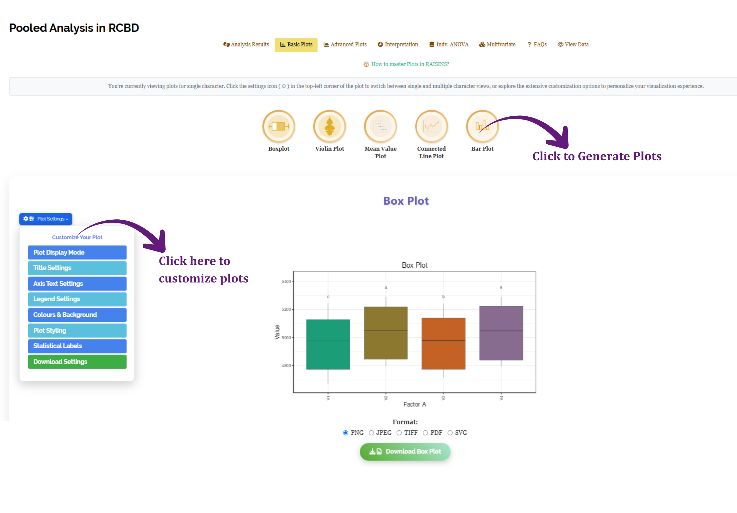
Numbers convince, but a picture persuades. Two dedicated tabs turn your results into publication-ready graphics. The Basic Plots tab offers a Boxplot, Violin plot, Mean value plot, Connected line plot, and Bar plot, each generated by clicking its icon. Every plot is fully customisable through the Plot Settings panel, display mode (single or multiple traits), titles, axis text, legend, colours, styling, and statistical labels, and can be downloaded in your chosen format. Use the Select Factor dropdown to plot by Treatment, Location, or their interaction. The box plot in Figure 11 carries the same a / b / c letter grouping as the treatment table: Dasheri on top, Kesar in the middle, Alphonso at the bottom.
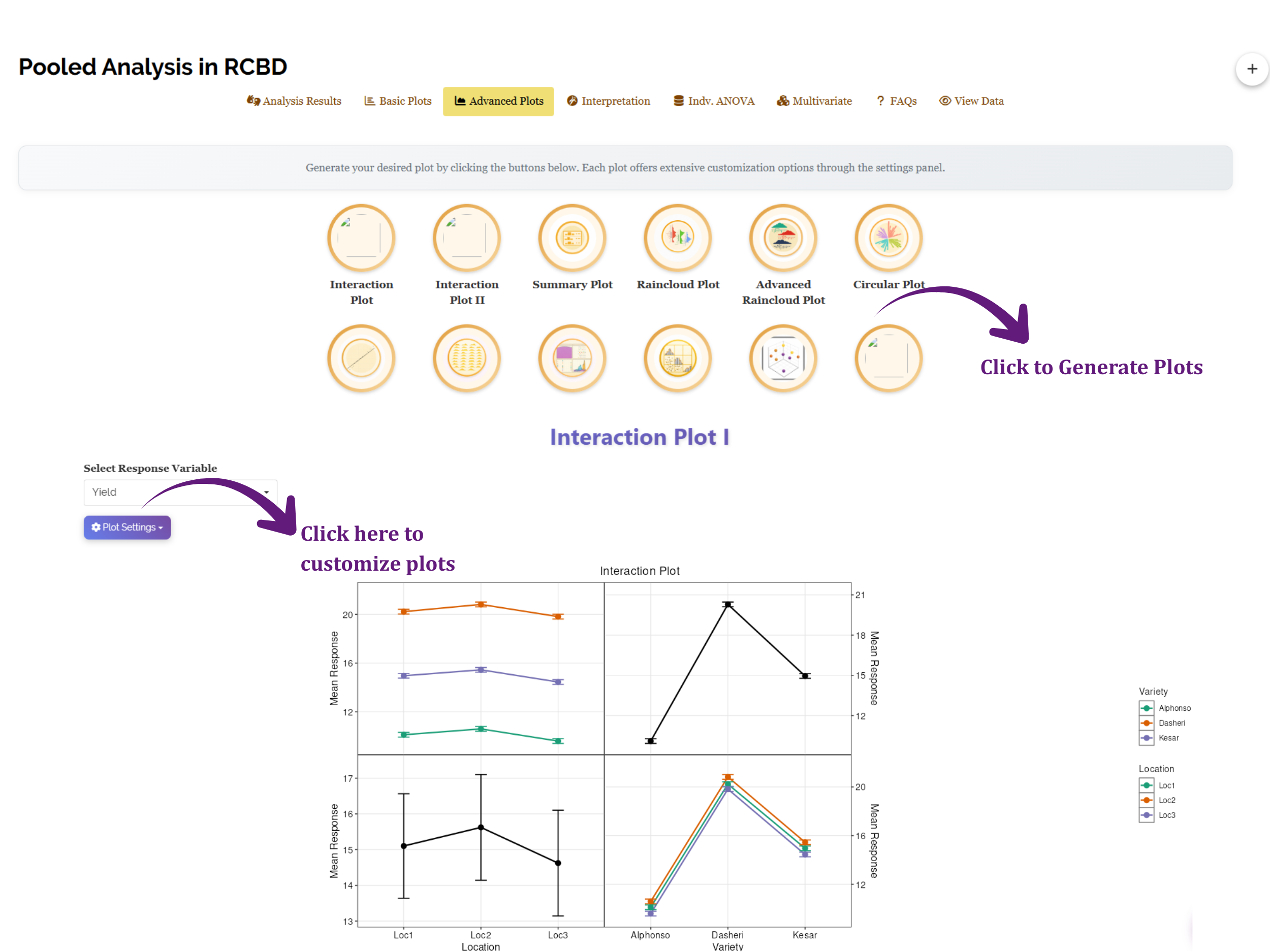
The Advanced Plots tab (Figure 12) goes further, with a Summary plot, Raincloud and Advanced raincloud, Circular, QQ, Distribution, Pair, and Correlation plots, and even 3D scatter and 3D scatter + line views for exploring several traits at once. These are especially useful for checking distributions and relationships between traits before you lean on the multivariate index (Section 19).
18 Individual ANOVA per environment
The pooled table answers the “across all environments” question. Sometimes you also want to see each environment on its own, exactly the individual RBD analyses that fed the pooling. The Indv. ANOVA tab provides them: a separate RBD ANOVA (with its own block, treatment, and error rows) and treatment-means table for each location, computed independently (Figure 13).
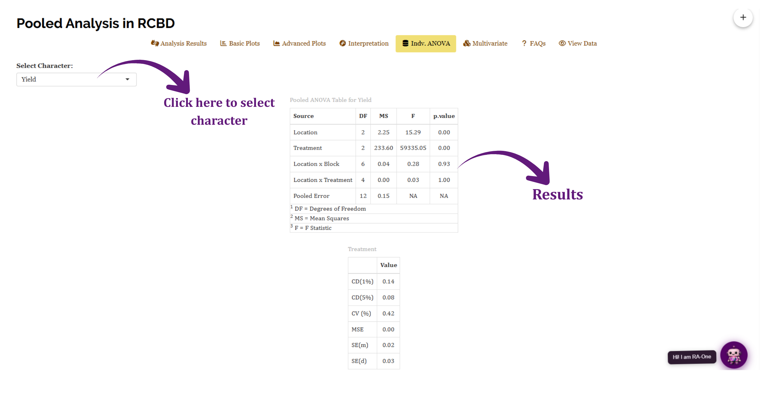
These per-location tables are most useful in two situations. First, when the interaction is significant and you can no longer quote a single overall winner, the individual analyses tell you which treatment won where. Second, as a diagnostic, if one location’s results look wildly different from the others, or its error is much larger, the individual view makes that obvious, and it is often the source of a significant Bartlett test. In the mango example, because the interaction was non-significant, the individual analyses simply echo the pooled conclusion at every location: Dasheri first, Kesar second, Alphonso third.
19 Multivariate: PCA index and correlation
So far each trait has been judged on its own. But a variety that is best for yield might not be best for sugar, and in a real recommendation you usually want a treatment that performs well across all traits at once. The Multivariate tab helps with this using Principal Component Analysis (PCA) and correlation analysis (Figure 14).
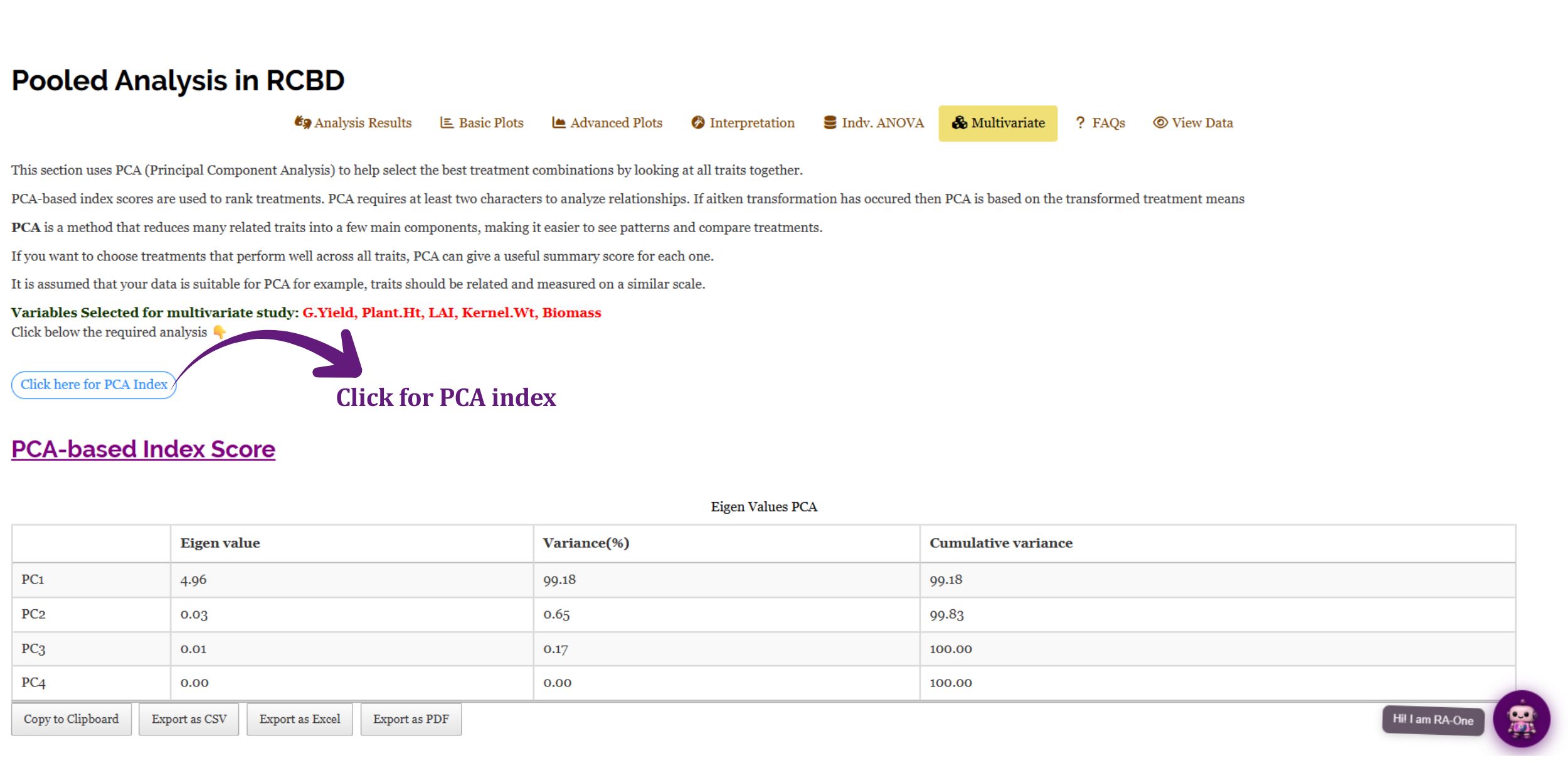
PCA reduces several related traits into a few underlying components, making it easier to see patterns and compare treatments. RAISINS uses the components to build a single index score for each treatment, a summary number that blends all the traits together, and ranks the treatments by it. This is handy when you want one overall “best across everything” answer rather than a separate winner per trait. If an Aitken transformation was applied, the PCA is based on the transformed treatment means. PCA requires at least two traits, since its whole purpose is to exploit the relationships between them.
The correlation analysis shows how the traits move together, whether high-yielding varieties also tend to have higher sugar, for example. Strong correlations tell you the traits carry overlapping information (and are good candidates for the PCA summary); weak correlations tell you each trait must be judged on its own.
Use the PCA index score for selection across multiple traits, when you must pick one treatment and every trait matters. Read it alongside, not instead of, the per-trait tables: the index tells you the best all-round performer, while the individual ANOVAs tell you exactly how it wins on each trait. In the mango example both agree, Dasheri leads on both traits, so it also tops the index.
20 Interpretation
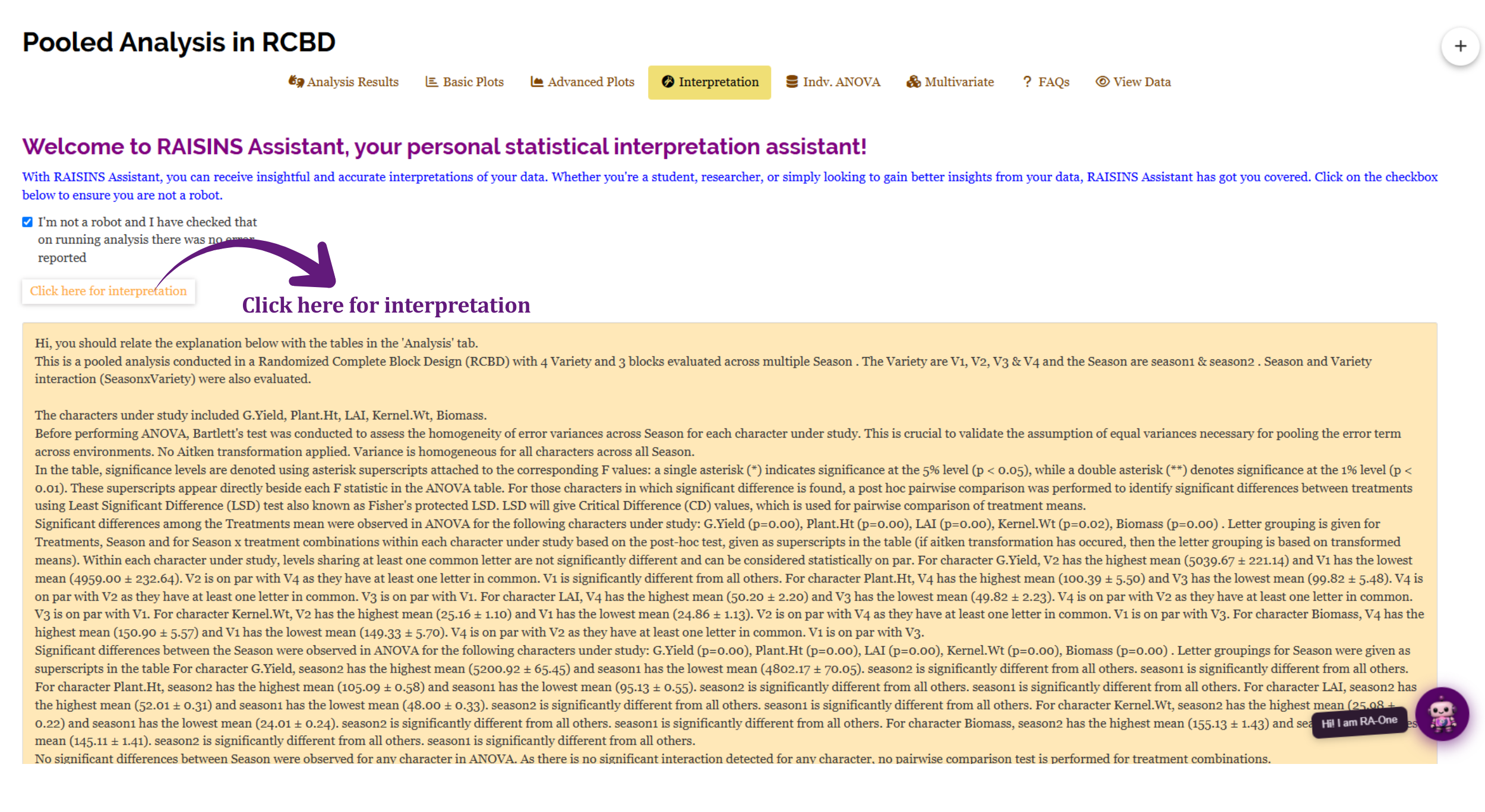
You do not have to translate the tables into prose yourself. The Interpretation sub-tab of the Analysis tab turns the pooled results into a clear, publication-ready narrative for each trait, stating whether the treatments differed, whether the environments differed, whether the blocking mattered, whether the interaction was significant, and which treatment came out on top, all in plain English (Figure 15). It is the fastest way to lift a defensible sentence straight into your thesis or report.
21 Chat with your data using RA-One
RA-One is the built-in conversational assistant for the Pooled RBD module, available from the RA-One tab. You ask questions in plain language and it answers using your own analysis rather than generic statistical advice. Every result it discusses is drawn from what the module actually computed, it never invents numbers, and if a value isn’t available it says so instead of guessing. All answers are in plain English, with no code or software commands.
RA-One works directly with your pooled ANOVA, Bartlett test, treatment and location means, and Interpretation outputs. It can explain whether the Location × Treatment interaction was significant for your data and what that means for your recommendation, tell you whether the blocking was worthwhile, walk you through why an Aitken transformation was or was not applied, tell you which variety was best for a given trait, and explain general concepts, what a critical difference is, how to read the letter grouping, why the error is pooled, so you build understanding alongside your results.
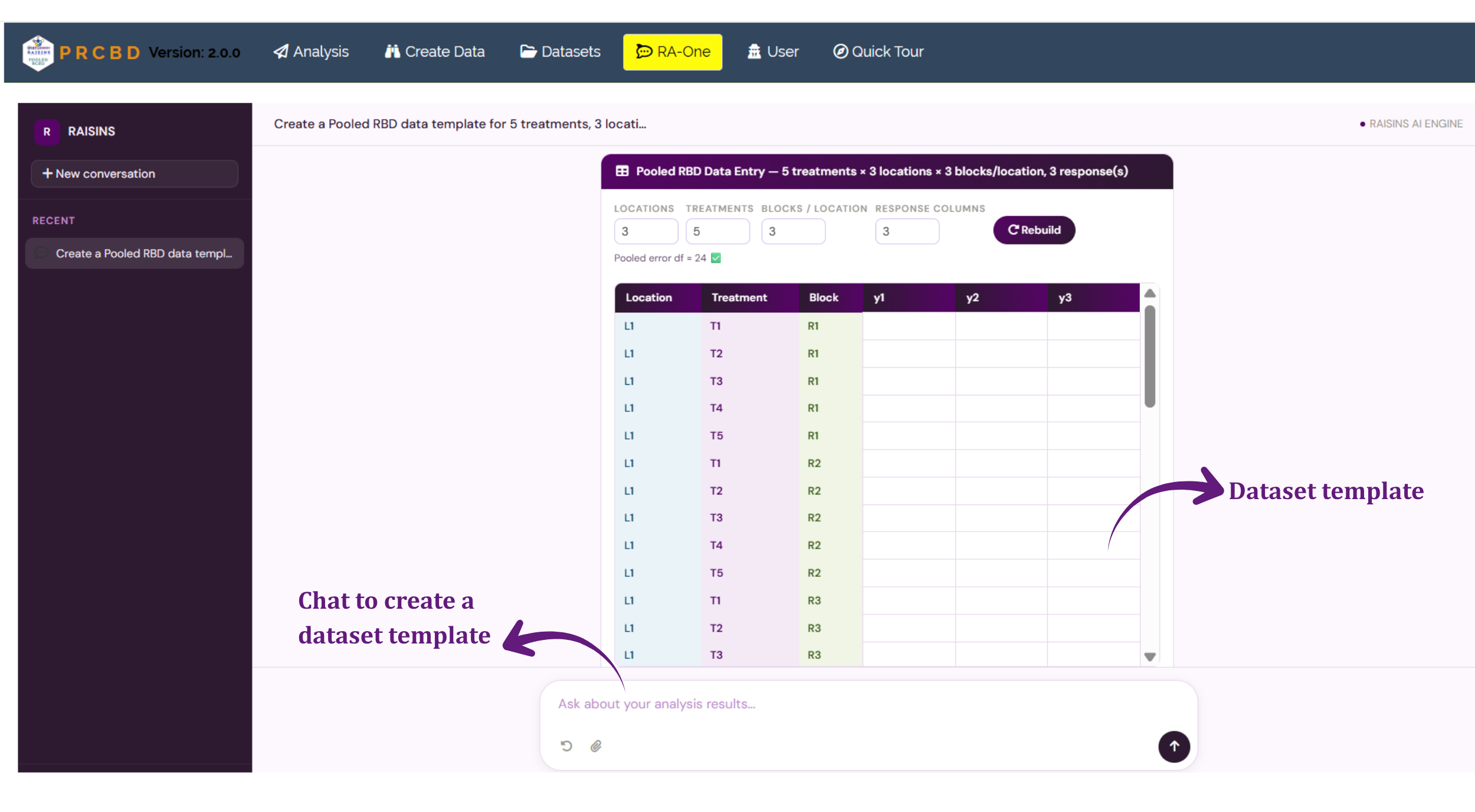
The same chat window can also prepare your data. It can build a correctly formatted pooled-RBD dataset template (Section 8.4) for you to fill in, or fetch a model dataset (Section 8.3) so you can try the module straight away, so you never need to leave the tab to get a file ready. RA-One can also generate plots on request, such as an interaction plot or a bar chart of treatment means, and render them directly in the chat, where you can refine them by asking for changes.
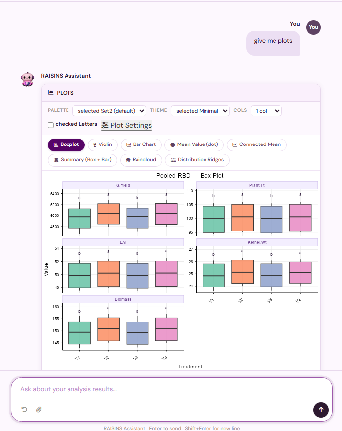
Within a single conversation, RA-One can interpret your pooled results, build a data template, fetch a model dataset, and produce plots, so most of a routine pooled-RBD session can be conducted without ever leaving the chat window.
22 FAQs
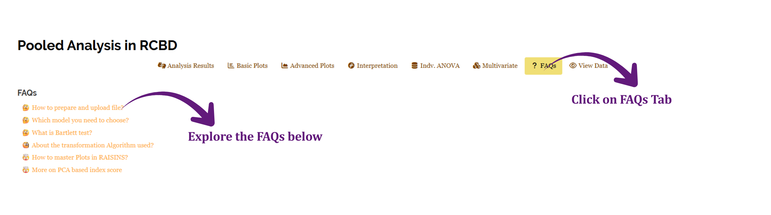
The module includes a dedicated FAQs section to clarify common doubts and guide you through the features. It offers detailed answers, additional information, and helpful tips for a smooth experience, including built-in explainers for what Bartlett’s test and the Aitken transformation do and how the PCA-based index score is built. If you are ever unsure how something works, say when the interaction changes your recommendation, or which multiple-comparison test to choose, the FAQs are a good place to start.
23 View data
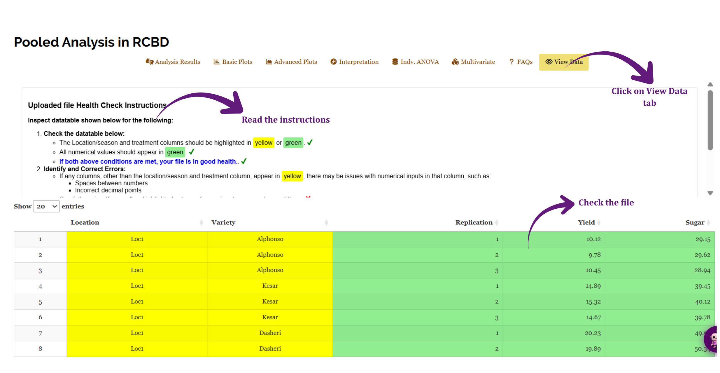
View Data is the primary diagnostic tool for ensuring data integrity before analysis. When you upload your dataset, the system performs an automated Health Check to validate column types and formatting. For a pooled RBD this step is especially important: it confirms that the environment, treatment, and block columns are read as categories, that every response variable column is numeric, that each treatment appears once in every block at every location, and that there are no missing or badly formatted entries that could distort the pooling.
24 Wrapping up
A pooled analysis in RBD rests on one honest question: does a treatment’s advantage hold up across environments, or only where it was tested? Everything else, the blocking, Bartlett’s test, the Aitken transformation, the interaction row, the individual analyses, exists to answer that question fairly. RAISINS automates the machinery, from checking that the experiments may be pooled to producing the pooled ANOVA and the treatment recommendation, so you can concentrate on what the answer means for your research.
If your design does not match a pooled RBD, the companion modules are there: the Pooled CRD module when your experiments had no blocking, the ordinary CRD and RBD modules for single-environment trials, and the factorial and split-plot modules for more structured designs. And if you get stuck at any point, RA-One is available 24 × 7, or write to us at [email protected].
