Randomized Block Design
A Randomized Block Design removes the variation caused by non-uniform field conditions, different days, or different batches by grouping similar experimental units into blocks. This tutorial explains what blocking buys you, how to read the RBD ANOVA table, when grouping letters appear, and how to run the whole analysis code-free in RAISINS… Read more …
The Randomized Block Design (RBD), also called the Randomized Complete Block Design (RCBD), is the workhorse experimental design of field research. When the experimental area is not uniform, or when material comes from more than one batch, treatments cannot simply be scattered at random without that variation contaminating the comparison. RBD solves this by grouping the experimental units into blocks of similar units and randomising the treatments within each block, so that the unwanted variation is measured and removed rather than left in the error term.
This tutorial explains what blocking does and why it makes a trial more sensitive, then provides a step-by-step guide to running the analysis in RAISINS without writing a single line of code: preparing your data, selecting the treatment and block columns, reading every row of the results table, choosing between LSD, Tukey’s HSD and DMRT, working through the thirteen available plots, running MANOVA and the PCA-based index score, and using the built-in RA-One AI assistant. Tables and plots are publication-ready.
1 What is a Randomized Block Design?
In a Completely Randomized Design (CRD), treatments are assigned to experimental units entirely at random. That is the right choice when every unit is essentially interchangeable, as in a laboratory or a growth chamber. In the field it is rarely true. One end of a plot may be wetter than the other, soil depth may change across a slope, and light may fall unevenly along a bench in a greenhouse. If treatments are scattered at random across ground like this, some treatments will be lucky and some unlucky, and that luck ends up inside the experimental error, inflating it and making genuine treatment differences harder to detect.
A Randomized Block Design (RBD) deals with this directly. The experimental area is divided into blocks, each block being a group of units that are as similar to one another as possible. Every treatment appears once in every block, and the allocation of treatments to units is randomised separately within each block. Because each block contains a complete set of treatments, the design is also called a Randomized Complete Block Design (RCBD).
Blocking does not remove the unwanted variation from your field; it removes it from your error term, by measuring it and accounting for it separately.
The pay-off is arithmetic. In a CRD, all variation that is not attributable to treatments is lumped into a single error sum of squares. In an RBD, that pool is split in two: the part that is systematically associated with the blocks, and what remains. The remainder becomes the new error mean square, and because it is smaller, the F-ratio for treatments is larger and the critical difference between two means is smaller. The same data, analysed with blocks recognised, is a more sensitive experiment.

The statistical model
Each observation is modelled as the sum of a grand mean, a treatment effect, a block effect and a random error:
\[y_{ij} = \mu + \tau_i + \beta_j + \varepsilon_{ij}\]
where \(\mu\) is the overall mean, \(\tau_i\) is the effect of the \(i\)-th treatment, \(\beta_j\) is the effect of the \(j\)-th block, and \(\varepsilon_{ij}\) is random error assumed to be independent and normally distributed with constant variance.
Notice what is absent: there is no treatment × block interaction term. The standard RBD analysis assumes that the treatments behave consistently from block to block, i.e. that block effects are additive. With one plot per treatment per block there is no replication within a block, so an interaction could not be estimated separately from error even if you wanted it. This is the single most important assumption of the design.
Two consequences follow from that model, and they shape everything in the results table:
- The block term is a nuisance factor. It is reported, and it is useful to look at, but the blocks are not what the experiment is about. RAISINS therefore does not run post-hoc comparisons between blocks.
- The treatment term is the hypothesis of interest. The null hypothesis is that all treatment means are equal; a significant F says at least one differs, and the post-hoc test then identifies which.
A significant block effect is good news, not a problem. It confirms that the ground really was variable and that blocking was worth doing. A non-significant block effect is not an error either, it simply means the area was more uniform than expected. Neither outcome invalidates the treatment comparison.
2 Blocking in Practice
The value of an RBD depends entirely on choosing the blocking factor sensibly. A block should capture the variation you expect, and units within a block should be as alike as possible while units in different blocks may differ freely.
Blocking factors commonly used in agricultural and biological research include:
- Position in the field, when there is a fertility, moisture or slope gradient. Blocks are laid out across the gradient, so that each block sits at a roughly constant level of it.
- Time, when the trial cannot all be run at once. Each day, week, or run of an instrument becomes a block.
- Batch or source, when material arrives from different seed lots, animals, or suppliers.
- Operator or instrument, when more than one person or machine takes the measurements.
- Every treatment must appear in every block, exactly once. That is what “complete” means in Randomized Complete Block Design.
- Randomise within each block, independently. Do not use the same treatment order in all blocks, that would confound treatment with position.
- Blocks should be internally homogeneous. A block that is itself half wet and half dry does no work.
- The number of blocks is the number of replications. Three or four is common in field trials; more blocks means more error degrees of freedom and a smaller critical difference.
If your design is not complete, for example there are too many treatments to fit a full set into any homogeneous area, RBD is not the right analysis and an incomplete block design should be used instead. If the experimental material genuinely is uniform and there is no blocking factor, use a Completely Randomized Design and the CRD module instead. Adding a meaningless block term simply costs degrees of freedom for nothing.
3 Getting to the Module
Open the RAISINS home page at www.raisins.live and go to the Analysis of Experiments section. Under Single Factor Experiments, select the RBD (Randomized Block Design) module (Figure 2).
No programming knowledge is required. You upload your data, choose which column holds the treatments and which holds the blocks, select one or more response variables, and RAISINS performs the complete analysis, from the ANOVA through the post-hoc comparison and compact letter grouping, and produces publication-ready output.

3.1 Computational Provenance & Reproducibility Record
CPRR (Computational Provenance & Reproducibility Record) provides a transparent and comprehensive record. Click on the icon shown in Figure 2 to access CPRR and know about the computational workflow performed during the analysis. The record for this module states the R version and the exact version of every package used, names the specific function behind each reported result. CPRR lists every default parameter and decision rule applied by the module and provides fully runnable R code that reproduces each analytical step. Users can execute the code in R to independently reproduce and verify the results. It carries its own DOI.
To cite the platform itself in a paper, thesis, or report, use the RAISINS citation, available in APA, Harvard, and BibTeX formats at www.raisins.live/citation.html. That is the primary reference, and for most manuscripts it is all you need.
The CPRR for the Randomized Block Design module is at www.raisins.live/module_record/rbd.html.
Cite the RAISINS paper as your primary reference for the platform. Add the CPRR as supporting documentation when a journal asks for details of the computing environment, or when you want your methods section to be precise about versions and functions rather than saying “analysis was carried out using an online tool.” The CPRR supports the citation and ensures computational reproducibility.
4 Preview Mode and Quick Tour
You can explore the entire module before subscribing by using Preview mode on the Welcome page. It loads the built-in demo datasets, so you can try every feature, including the analysis, the post-hoc comparisons, the multivariate section and all thirteen plots, without uploading your own data. Uploading your own file is the only action disabled in preview mode.
On first login you are also offered a choice between Take the tour and Skip. Taking the tour launches an interactive, guided walkthrough of nineteen steps that highlights each navbar tab, each analysis subtab and the sidebar in turn and explains what it does, from uploading a file all the way through to logging out. You can replay it at any time from the Quick Tour tab in the top navigation, whether or not you took it the first time.

5 The Example Dataset
This tutorial uses the built-in Mango Variety Data (dataset1.csv), available from the Datasets tab. It is a hypothetical evaluation of ten mango varieties grown in three blocks, giving 30 rows in total. The varieties are Alphonso, Kesar, Dasheri, Himsagar, Chausa, Badami, Safeda, Bombay_g, Langra and Totapuri. Because every variety appears once in each of the three blocks, the number of blocks is also the number of replications per treatment.
Four response variables were recorded on each plot:
- yield
- Obs1
- Obs2
- FW (fruit weight)
The file is laid out with a Treatment column first, a Block column second, and the four response columns after that, one per measured trait (Figure 4).

Two terms recur throughout this tutorial. Treatments are the things being compared, here the mango varieties. Variables, sometimes called characters or traits, are the measurements taken on each plot, here yield, Obs1, Obs2 and FW. The Block column is neither of these; it records which block each plot belonged to.
- Prepare your dataset.
- Upload the data.
- Select the Treatment column, the Block column, and one or more Variables.
- Apply a transformation if the data need one.
- Click Run Analysis.
- Choose the multiple comparison test, p-adjustment, significance level and digits.
- Read the ANOVA table and the main results table with its grouping letters.
- Review the summary statistics, the trait-wise ANOVA, and the plots.
- Run the multivariate analysis if you have several traits.
- Read the automatic interpretation, or ask RA-One.
- Export the downloadable report.
The sections below walk through each of these steps in detail.
6 Preparing Your Data
The quality of your analysis depends on the quality of your data. RAISINS provides four ways to prepare a correctly formatted dataset:
- Create it in MS Excel.
- Build it inside the app using Create Data.
- Download a built-in Model dataset and use it as a reference.
- Generate it through the RA-One chat assistant.
6.1 Preparing Data in MS Excel
Open a new Excel workbook containing a single sheet. Arrange the data in columns: one column for the Treatment labels, one column for the Block number, and then one column for each numeric response variable. Each row is one experimental unit, that is, one treatment in one block. Every response column must contain only numeric values.
Save the file in CSV, XLS or XLSX format. CSV is recommended because it is smaller and loads faster. Avoid blank rows above the data and extra spaces in column names. Refer to Figure 4 for the required layout.
Every row must carry a block label, and every treatment must appear exactly once in every block. If a treatment is missing from a block, or appears twice in the same block, the design is no longer a complete block design and the ANOVA will not be correct. Check this before uploading; the View Data tab (Section 17) will help you confirm it.
Dataset creation rules
- Column naming - do not use spaces. Use underscores (
_) or dots (.), and avoid symbols such as % and #. Always begin a column name with a letter. - Data arrangement - start at the upper-left corner of the sheet. The row above the data must not be blank.
- Cell management - do not type or delete in empty cells. If needed, select them, right-click, and choose Clear Contents.
- Column relevance - give every column a meaningful name, and remove columns you will not analyse.
- Consistent labels -
Alphonsoandalphonso(with a trailing space) are read as two different treatments. Keep the spelling identical throughout. - Numeric response columns only - every response variable column must contain only numbers. Entries such as “NA” or ” - ” will cause errors. The Treatment and Block columns are the only columns allowed to hold labels.
How to save as CSV in MS Excel
- Open your workbook, with the data on a single sheet and correctly arranged.
- File → Save As / Save a Copy, then choose a location.
- Save as type → CSV (Comma delimited) (*.csv).
- Name the file without spaces. Use underscores instead.
- Save.
💡 Tip: before saving, confirm that the data is on the first and only sheet, that the Treatment and Block columns come first, and that every response column is numeric.
6.2 Creating Data Inside RAISINS
If you are unsure about the required format, RAISINS can generate a correctly structured template for you:
- Go to the Create Data tab.
- Enter the number of treatments (2 to 100).
- Enter the number of Blocks (2 to 100).
- Enter the number of characters to analyze (1 to 100).
- Click Create.
The generated layout is shown in Figure 5, already carrying the correct Treatment and Block columns with every treatment repeated once per block. Enter your observations directly into the template, or download it as a CSV file, fill it in, and upload it in the Analysis tab.

6.3 Downloading Model Datasets
To explore the module before using your own data, download one of the three ready-made examples from the Datasets tab:
- Mango Variety Data - 10 mango varieties in 3 blocks, with yield, Obs1, Obs2 and FW. This is the dataset used throughout this tutorial.
- Chemical Data - 4 chemical treatments (C1 to C4) in 4 blocks, observed on Day1, Day3, Day6, Day7 and Day15. Its final column holds proportions, so it is useful for testing the arcsine transformation.
- Water Quality Data - 5 river stations treated as treatments, with three observation points each, recording transparency, depth, air and water temperature and pH.
Use any of them as a formatting reference, or upload one directly to run the analysis.

6.4 Creating a Dataset Using RA-One
RA-One, the built-in chat assistant, can create a correctly formatted dataset through a simple conversation.
Open RA-One from its navigation tab or from the floating chat bubble in the bottom-right corner. Tell it how many treatments, how many blocks and how many response variables you need, and it generates a template in the required format, Treatment and Block columns first, response columns after. Review the template in the chat, download the CSV file, and upload it in the Analysis tab (Figure 7).
RA-One can also advise on how many blocks your trial should have before you lay it out. Ask it something like “how many replications do I need for 8 treatments?” and it will answer with the error degrees of freedom that choice would give you.

7 The Analysis Tab
The top-level navigation of the module runs Welcome, Analysis, Create Data, Datasets, RA-One, User, Quick Tour, in that order. Everything from here through Section 17 happens inside Analysis, which is itself organised into nine subtabs shown as pills across the top of the page: Analysis Results, Summary stats, Individual ANOVA, Basic Plots, Advanced Plots, AI interpretation, Multivariate, FAQs, View Data.
Upload your prepared file by clicking Browse in the sidebar. As soon as the file is read, three selectors appear:
- Select the treatment - the column holding the treatment labels.
- Select the blocks - the column holding the block or replication number.
- Select variables - one or more response columns. You can select them all at once and the module analyses each in turn.
The three lists are linked: a column you have already assigned as the treatment disappears from the block and variable lists, so the same column cannot be used twice.

Below the selectors is the transformation switch (Section 7.1). Once you click Run Analysis, the results appear immediately, and a row of controls appears above the results table:
| Control | Choices | Default |
|---|---|---|
| Multiple comparison test | LSD, TUKEY, DMRT | LSD |
| P-adjustment (LSD only) | None, Bonferroni (FWER), Holm-Bonferroni (FWER), Benjamini-Hochberg (FDR) | None |
| Level of significance (α) | 0.05, 0.01 | 0.05 |
| Digits after decimal | 1 to 4 | 2 |
| Font | several typefaces for the output tables | - |
Changing any of these updates the tables and plots at once; there is no need to re-run the analysis. Two further toggles sit directly above the table, one to show or hide the ± SD alongside each mean, and one to show or hide the grouping letters.
7.1 Transformation
ANOVA assumes that the errors are normally distributed with constant variance. When a variable is a count, a proportion, or is strongly right-skewed, that assumption may fail, and a transformation applied before analysis can restore it. Switch on the transformation option in the sidebar and choose, per variable, one of three transformations (Figure 9).
Logarithmic replaces each value with log10(x). It suits positive, continuous data whose spread grows in proportion to the mean, which is typical of multiplicative or exponential processes. If any value is zero or negative, RAISINS shifts the data first and applies log10(x - min(x) + 1), so the transformation never fails on your data.
Square root replaces each value with sqrt(x). It is the standard choice for count data, where the variance rises with the mean, as in a Poisson process. If any value is exactly zero, RAISINS uses sqrt(x + 0.5) instead. Negative values are rejected, since their square root is undefined.
Arcsine, also called the angular transformation, replaces each proportion with asin(sqrt(x)). It applies to data bounded between 0 and 1, and stretches the two ends of the scale where the binomial variance is naturally smallest. Exact zeros and ones are replaced by 1/(4n) and 1 - 1/(4n) respectively before the transformation, following the usual convention.

When a transformation is applied, the ANOVA is run on the transformed values, because that is where the assumptions hold. The results table then shows the original mean with the transformed mean in parentheses beneath it, so you can report the familiar scale while the test statistics come from the transformed analysis. Report both, and say which transformation you used.
8 Analysis Results
Clicking Run Analysis fits, for each selected variable, the blocked linear model
\[\text{variable} \sim \text{Treatment} + \text{Block}\]
and produces two tables.
8.1 The ANOVA table
The first table is the classical analysis of variance summary. It has one row per source of variation, Treatment, Block and Error, a DF column, and then one column per response variable holding that source’s mean square. Significance is marked as a superscript on the mean square: ** at the 1% level, * at the 5% level, and NS when not significant (Figure 10).

For yield, the treatment mean square (40376.08) is roughly five times the error mean square (8191.51), giving F = 4.93 on 9 and 18 degrees of freedom, significant at the 1% level (p = 0.0020). At least one variety differs in yield. The block mean square (32597.00) gives F = 3.98, p = 0.0371, significant at 5%: the three blocks really did differ, so blocking was worthwhile here and removing that variation sharpened the treatment test.
For Obs1 the treatment effect is significant at 5% (F = 3.38, p = 0.0134) while the block effect is not (p = 0.2221). For Obs2 (p = 0.1437) and FW (p = 0.4201) neither term is significant, so for those two traits there is no evidence that the varieties differ at all.
Note the degrees of freedom, since they are the clearest signature of an RBD. With t treatments and r blocks, treatments carry t − 1 df, blocks carry r − 1 df, and error carries (t − 1)(r − 1) df. In this example that is 9, 2 and 18, adding to 29, one less than the 30 observations. A CRD on the same 30 plots would have given error 20 df; the RBD trades two of them to the block term, and gets a smaller error mean square in return.
8.2 The main results table
The second table is the one you will put in a paper. Its columns are the response variables and its rows are, first, one row per treatment carrying the treatment mean ± SD with the grouping letter as a superscript, followed by a block of summary rows (Figure 11):
- F stat - the treatment F-ratio, with its significance star.
- p value - the exact p-value for the treatment effect.
- CD - the critical difference (also called LSD), or the equivalent critical value for whichever post-hoc test you selected.
- MSE - the error mean square.
- SE(m) - the standard error of a treatment mean,
sqrt(MSE / r). - SE(d) - the standard error of the difference between two treatment means,
sqrt(2 × MSE / r). - CV(%) - the coefficient of variation, a measure of experimental precision.
- Cohen’s F - the effect size for the treatment term.
Here r is the number of blocks, since that is how many times each treatment was replicated.

If the treatment p-value is greater than the selected α, RAISINS blanks the grouping letters and prints “-” in the CD row for that variable. This is deliberate. A post-hoc test is only meaningful after the omnibus F has rejected the null hypothesis; reading pairwise letters from a non-significant ANOVA inflates the Type I error rate.
In this example that means yield and Obs1 carry letters, while Obs2 and FW show none. Note also that the stars use fixed 0.01 and 0.05 thresholds while the letters are gated on the α you selected, so at α = 0.01 a variable with p = 0.03 would still show a * but would carry no letters.
For yield, Alphonso recorded the highest mean (1423.92 ± 110.44) and Safeda the lowest (1061.19 ± 149.30). With a critical difference of 155.26, Alphonso is statistically on par with Dasheri (1369.90) and Totapuri (1335.17), and also with Badami and Chausa, all of which share a letter with it. Safeda shares its letter with Langra, Kesar, Bombay_g and Himsagar. Treatments that share no letter, such as Alphonso and Safeda, differ significantly at the 5% level.
The coefficient of variation for yield is 7.30%, which is low for a field trial and indicates good experimental precision. Cohen’s f for the treatment term is 1.57, far above the 0.40 threshold conventionally taken as a large effect, so the variety differences are not only statistically detectable but substantial.
8.3 Reading the grouping letters
Letters summarise all pairwise comparisons at once. Treatments that share at least one letter are not significantly different, or “on par”. Treatments with no letter in common differ significantly. Overlapping labels such as ab or bcd are normal, they mean that treatment is indistinguishable from members of more than one group. Letters are assigned in order of decreasing mean, so a always marks the top group.
8.4 Multiple comparison tests
Once the ANOVA is significant, a post-hoc test identifies which specific pairs of treatments differ. All three options in RAISINS use the pooled error mean square and error degrees of freedom from the blocked model, so the block adjustment carries through into the pairwise comparisons.
The three post-hoc tests
LSD (Least Significant Difference) computes a single critical difference
\[\text{CD} = t_{\alpha/2,\ df_{error}} \times \sqrt{\frac{2\ \text{MSE}}{r}}\]
and declares any two means differing by more than that to be significantly different. It is the most sensitive of the three and the most widely used in agricultural research, but because it applies the same threshold to every pair without adjustment, the family-wise error rate rises as the number of treatments grows.
Tukey’s HSD (Honestly Significant Difference) replaces the t value with the studentised range statistic, which is calibrated for the largest difference among t means. It controls the family-wise error rate across all pairwise comparisons, making it the conservative and safe choice when there are four or more treatments and you intend to compare them all.
DMRT (Duncan’s Multiple Range Test) ranks the means and uses a critical range that widens with the number of means spanned by the comparison. It detects more differences than Tukey’s HSD and is popular in agricultural work, at the cost of a higher Type I error rate. When DMRT is selected, RAISINS additionally displays the table of critical ranges used.
When LSD is selected, a P-adjustment control appears offering Bonferroni, Holm-Bonferroni and Benjamini-Hochberg corrections. Choosing any of them changes what can be reported: a single critical difference is no longer defined once each comparison carries its own adjusted threshold, so the CD and p value rows are removed from the table and the adjusted result is carried entirely by the grouping letters. This is expected behaviour, not a missing value.
The choice is yours to justify, not the software’s. LSD is conventional in agronomy and is most defensible with a small number of treatments or a small set of planned comparisons. Tukey’s HSD is the right choice when you are comparing all pairs among many treatments and want strict error control. DMRT sits between them. Whichever you choose, state it in your methods section along with the significance level.
9 Summary Statistics
The Summary stats subtab gives one table per response variable, describing each treatment in its own right rather than in comparison with the others (Figure 12). Each table has one row per treatment and the following columns:
- Mean - the arithmetic average across the blocks.
- SD - the standard deviation, a measure of spread.
- SE - the standard error of the mean,
SD / sqrt(n). - Min and Max - the lowest and highest observed values.
- CV - the coefficient of variation,
SD / Mean × 100, which allows spread to be compared across traits measured on different scales. - Skewness - the asymmetry of the distribution. Positive means a long right tail, negative a long left tail.
- Kurtosis - the tailedness of the distribution.
These are descriptive statistics computed from the raw observations. They do not use the pooled error term, so the SE here is not the same quantity as the SE(m) in the main results table, which is derived from the MSE. Use SE(m) when reporting treatment means from the model, and this table when describing the raw data.

10 Individual ANOVA
The main results table compresses each variable into a single column. The Individual ANOVA subtab expands one trait at a time into a full, conventional ANOVA table, which is what most theses and journals expect to see (Figure 13). For the selected trait it reports:
- The complete ANOVA table with Source (Treatment, Block, Residuals), DF, SS, MS, F and p-value.
- A treatment summary with means and grouping letters.
- The critical difference at both the 5% and the 1% level, so you can report either without re-running the analysis.
- MSE, SE(m), SE(d) and CV(%).
The post-hoc method and p-adjustment you selected in Analysis Results apply here too. Each table can be downloaded, and there is a separate trait-wise report download for this subtab.

11 Plots and Graphs
Thirteen plot types are available across two subtabs. Each is chosen by clicking its icon, and each opens with a gear icon that reveals a full customisation panel: titles, axis labels, colour palettes, fonts, point sizes, error bar style, and whether the grouping letters are drawn. Every plot can be downloaded as PNG (300 dpi), JPEG, TIFF, PDF or SVG, ready for a manuscript or a presentation.
11.1 Basic Plots
The Basic Plots subtab holds the five treatment-comparison plots. All five carry the grouping letters from the post-hoc test, so each one is a visual version of the results table (Figure 14).
- Boxplot - shows the median, interquartile range and any outliers for each treatment. The best first look at whether the spread is comparable across treatments.
- Violin Plot - a boxplot wrapped in a density curve, so you can see the shape of the distribution as well as its summary.
- Bar Plot - treatment means as bars with error bars. The familiar format for agronomy papers.
- Mean Value Plot - treatments listed down the side with their means as points and horizontal error bars. Easier to read than a bar chart when there are many treatments.
- Connected Line Plot - treatment means joined by a line, useful when the treatments have a natural order such as increasing dose or date.

The comparison plots display the raw treatment means and their observed spread, while the letters on them come from the post-hoc test, which does use the block-adjusted error term. The two are consistent for a balanced complete block design, which is what this module analyses, but it is worth knowing that the error bars and the letters are computed from different quantities.
11.2 Advanced Plots
The Advanced Plots subtab holds eight further displays, aimed at understanding distributions, checking assumptions and exploring relationships between traits (Figure 15).
- Summary Plot - a compact overview of how each variable is distributed.
- Raincloud Plot - a half-violin density “cloud” with the individual observations shown as “rain” beneath it. This is a pooled marginal view of the variable.
- Advanced Raincloud Plot - the same idea drawn per treatment, combining density, boxplot and raw points so you can compare full distributions rather than just means.
- Circular Plot - treatment values drawn radially, an attractive layout when there are many treatments to display at once.
- QQ Plot - observed quantiles against the quantiles of a normal distribution. Points close to the diagonal indicate approximate normality; systematic curvature suggests a transformation may help.
- Distribution Plot - the spread of values within each treatment.
- Pair Plot - a matrix of scatterplots for every pair of response variables, with correlations, useful before deciding whether a multivariate analysis is worthwhile.
- Correlation Plot - the correlation matrix among the response variables, shown graphically.

The RBD ANOVA assumes normally distributed errors with constant variance. The QQ plot is the quickest visual check on the first, and the Boxplot on the second: if the boxes have wildly different heights, the constant-variance assumption is in doubt and a transformation (Section 7.1) is worth trying.
12 Multivariate: MANOVA and the PCA Index
When several traits have been measured on the same plots, testing each one with its own ANOVA answers “does variety affect yield?” separately from “does variety affect fruit weight?”. The Multivariate subtab answers the combined question: do the varieties differ when all traits are considered together?
Two analyses are provided. Both require at least two response variables, and the number of treatments must be greater than the number of response variables.
12.1 MANOVA
Multivariate analysis of variance fits the same design to all the response variables at once, cbind(traits) ~ Treatment + Block, and reports Pillai’s trace together with its approximate F, the numerator and denominator degrees of freedom, the p-value, and partial η² as an effect size, for both the treatment and the block term (Figure 16).

Taking all four traits jointly, the varieties differ significantly (Pillai’s trace = 2.08, F = 2.17 on 36 and 72 df, p = 0.0027), with a partial η² of 0.52. The block term is not significant in the multivariate test (p = 0.284, partial η² = 0.24), even though it was significant for yield alone. That is a useful reminder that a multivariate test asks a different question from a stack of univariate ones, and the two need not agree.
12.2 PCA-based Index Score
MANOVA tells you whether the treatments differ overall. It does not tell you which treatments are best. For that, RAISINS builds an index score from a principal component analysis of the treatment means. Click the PCA button to run it, and four pieces of output appear in turn.
Eigenvalues. The variance explained by each principal component, individually and cumulatively. In the example, PC1 accounts for 41.16% of the variation among the treatment means and PC2 for 29.50%, together explaining 70.66%. A scree plot shows the same information graphically.
Loadings. How each original variable contributes to each component, and therefore what each component means. In the example, PC1 has positive loadings for yield (0.498) and Obs2 (0.657) but negative loadings for Obs1 (−0.131) and FW (−0.551). A treatment with a high PC1 score is therefore high in yield and Obs2 and low in FW. PC2 loads mainly on Obs1 (0.826) and yield (0.533).
Biplot. Treatments and variable vectors drawn in the same plane. A treatment sits in the direction of the variables it scores highly on, and the angle between two variable arrows reflects their correlation: a small angle means a strong positive correlation, a right angle means little correlation.
Index score. Each treatment’s score on the chosen component, and a scaled index rescaled to run from 0 to 1 so that treatments can be ranked and compared easily. Set a cutoff, 75% by default, and use the up and down arrows to select the top or the bottom percentage of treatments. Selected treatments are highlighted in yellow in the table and marked on the accompanying index plot.
Look at the loadings before you choose. If the traits you want to improve all load positively on PC1, rank treatments by a high PC1 index. If they load negatively, rank by a low PC1 index instead. If PC1 explains little and the traits you care about load on PC2, base the index on PC2. As a rough guide, a PC1-based index is well supported when PC1 alone explains more than about 40% of the variance, and a two-component index when the first two together exceed roughly 60%.
Remember that PCA is exploratory, not inferential. The index score ranks treatments; it does not test them. The formal test of treatment differences remains the ANOVA and the MANOVA.
13 Interpretation
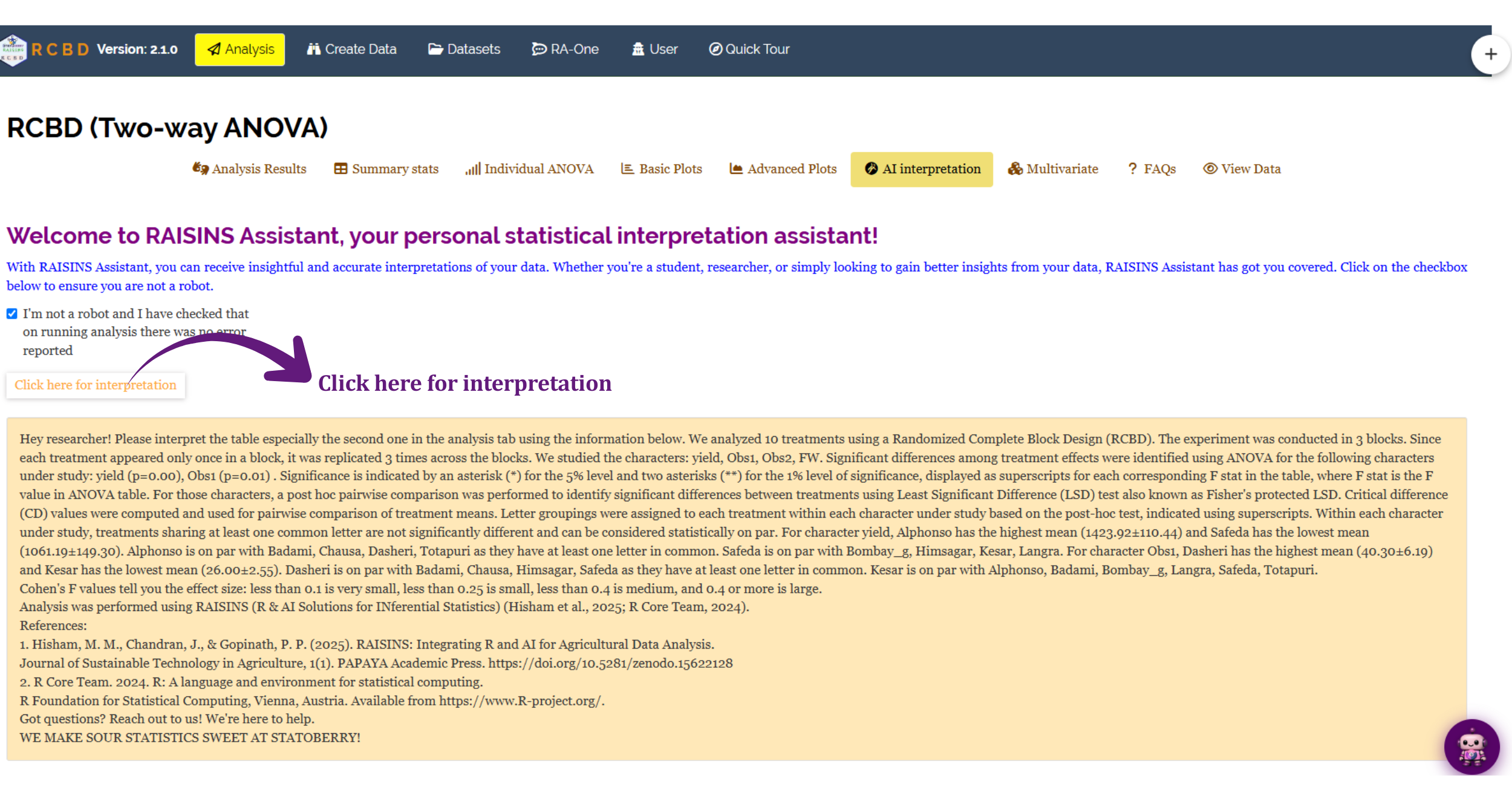
The AI interpretation subtab turns the numerical output into readable prose. Select the variables you want covered, click the button, and RAISINS produces a written account of the analysis: which treatments differed, how the grouping letters should be read, what the coefficient of variation says about the precision of the trial, and what the effect size implies about the practical importance of the differences (Figure 17).
Treat it as a well-informed first draft. It reads the numbers correctly, but it does not know your agronomy, your site or your objectives. Check it against what you know about the experiment before using any of it in a manuscript.
14 RA-One Chat Assistant
RA-One is the module’s conversational assistant. It is available from its own navigation tab and from the floating chat bubble in the bottom-right corner of every page, so you can ask a question without losing your place in the analysis.
Unlike a general-purpose chatbot, RA-One can see the analysis you have just run. Once you have clicked Run Analysis, it has access to your ANOVA results, treatment means, grouping letters and precision statistics, so you can ask about your own numbers rather than about statistics in the abstract (Figure 18).
Useful things to ask it:
- Design questions before you start. “How many blocks do I need for 8 treatments?” or “should I block by field position or by day?”
- Data preparation. “How should my file be laid out?” or “make me a template for 6 treatments in 4 blocks with 3 traits”, which produces a downloadable CSV.
- Model datasets. Ask for an example dataset and it will point you to the right one.
- Result interpretation. “Why does Obs2 have no letters?” or “what does a CV of 7.3% mean here?” or “is the block effect important?”
- Method choice. “Should I use Tukey or LSD for ten treatments?”

The first time you open RA-One after running an analysis, a consent dialog explains that your analysis results are sent to a large language model to generate the answer, and what that means for your data. Read it before accepting. If you are working with unpublished or sensitive results, use the rest of the module, which is entirely local to the R session, and skip the assistant.
15 Downloadable Report
Everything you have generated can be exported as a single formatted document. Choose HTML, PDF or Word and click download. The report assembles the ANOVA table, the results table with its grouping letters, the summary statistics and the plots, laid out and captioned, so it can be attached to a thesis chapter or circulated to collaborators as it is. The Individual ANOVA subtab has its own separate report download for trait-wise output.
Individual tables and plots can also be downloaded on their own from the subtab where they appear, if you would rather assemble the document yourself.

16 FAQs
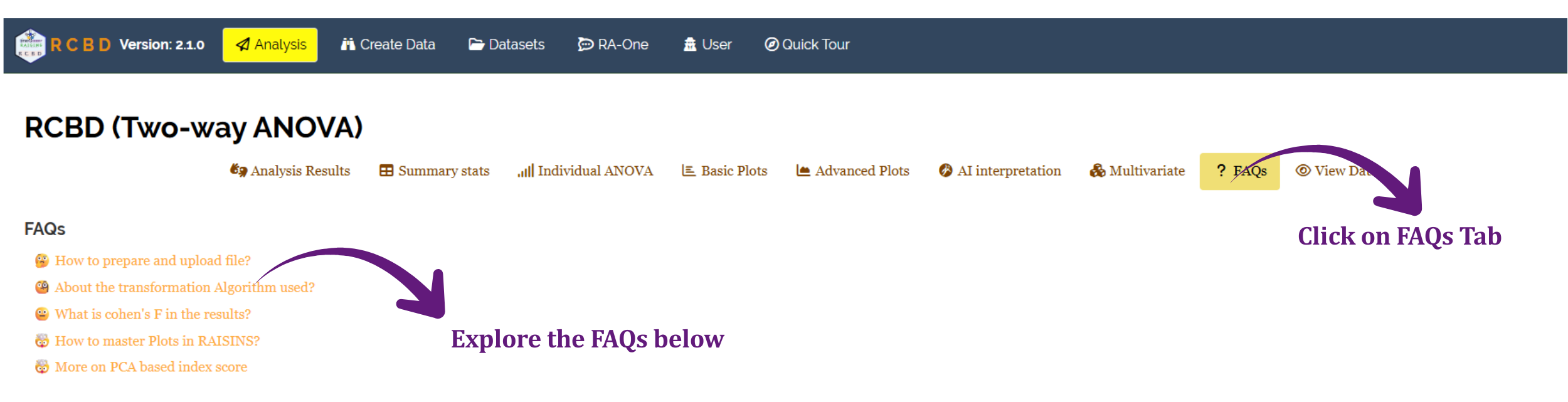
The FAQs subtab collects answers to the questions that come up most often, on file formats, on the difference between the post-hoc tests, on when to transform, and on how to read the grouping letters. If something in the module is not behaving as you expect, start here.
17 View Data
View Data is the diagnostic tool to reach for before, not after, something goes wrong. It displays the uploaded file exactly as RAISINS has read it, and runs an automated health check on the column types and formatting.
For an RBD in particular, use it to confirm two things: that the Block column has been read as a label and not accidentally as a measurement, and that every treatment appears once in every block. A stray extra row, a misspelled treatment name, or a missing plot will show up here immediately, whereas in the results table it would only appear as a puzzling degree-of-freedom count.

18 Summary
A Randomized Block Design earns its keep whenever the experimental material is not uniform. By grouping similar units into blocks and randomising treatments within each block, the variation you cannot control is measured and set aside rather than being left to inflate the error term.
In RAISINS the whole workflow is code-free. Upload the file, name the treatment and block columns, choose the response variables, and click Run Analysis. The ANOVA table separates treatment, block and error; the results table carries the treatment means, grouping letters, critical difference and precision statistics; the trait-wise ANOVA gives the conventional layout a thesis expects; thirteen plots visualise the comparison and check the assumptions; MANOVA and the PCA index handle several traits at once; and RA-One and the automatic interpretation help you explain what you are looking at. Every table and plot is publication-ready, and the whole analysis exports as a single report.
The two things worth carrying away are these. First, the letters mean nothing unless the ANOVA is significant, which is why RAISINS hides them when it is not. Second, a significant block effect vindicates the design; it is evidence that blocking removed real variation, and it belongs in your results, not in a footnote.
19 Appendix: A Short History of the Randomized Block Design
The randomized block design was developed by Ronald A. Fisher at Rothamsted Experimental Station during the 1920s, alongside the analysis of variance itself. Fisher’s insight was that the two problems facing field experimentation, systematic soil variation and the need for a valid estimate of error, could be solved together. Grouping plots into blocks handled the first; randomising within blocks guaranteed the second, by ensuring that the error term really did estimate random variation rather than a hidden pattern.
The design was set out in Statistical Methods for Research Workers (1925) and, more fully, in The Design of Experiments (1935), and it spread from Rothamsted’s field plots into essentially every experimental science. A century on, it remains the default layout for varietal trials, fertiliser experiments, greenhouse studies and laboratory work run in batches, for the same reason Fisher introduced it: it is the simplest design that both controls a known source of variation and still yields an honest estimate of error.
