Split-Split Plot Design
A split-split-plot design handles three factors when they must be applied to progressively smaller experimental units, splitting the experiment into whole-plot, subplot, and sub-subplot strata with an error term for each. This tutorial explains where the design comes from, why it needs several different critical differences, and how to run the whole analysis in RAISINS… Read more …
Split-split-plot designs extend the split-plot idea to three treatment factors whose levels differ in how easy they are to change during the experiment. The hardest-to-change factor is assigned to whole plots, the next to subplots nested inside each whole plot, and the easiest-to-change factor to sub-subplots nested inside each subplot. RAISINS fits the appropriate three-stratum model, reports all three error terms and every associated critical difference, provides post-hoc letter groupings for every interaction, and presents a plain-language interpretation of the results, all without requiring you to write a single line of code. This tutorial will guide you through the analysis step-by-step.
1 What is a split-split-plot design?
A split-split-plot design is used when three treatment factors are studied together, but the three differ in how easy they are to apply or change from one plot to the next. The factor that is hardest to change is assigned to whole plots, the next-hardest factor is assigned to subplots nested inside each whole plot, and the factor that is easiest to change is assigned to sub-subplots nested inside each subplot.
Consider an experiment comparing two irrigation methods, two fertilizer doses, and two crop varieties. Irrigation method is the hardest to change, sprinkler and drip systems are typically laid out over a sizeable area and cannot easily be alternated plot by plot. Fertilizer dose can be varied within an irrigation area, but still requires a reasonably sized strip to apply cleanly. Variety, by contrast, can be sown in whatever small plot you like. Randomising all \(2 \times 2 \times 2 = 8\) treatment combinations independently to the smallest plots would be impractical, because the irrigation method cannot physically be switched on and off between neighbouring one-metre plots.
A split-split-plot design addresses this constraint through three stages of randomisation. First, the hardest-to-change factor is randomly assigned to the whole plots. Each whole plot is then divided into subplots, and the next factor is randomly assigned within those subplots. Each subplot is divided again into sub-subplots, and the easiest-to-change factor is randomly assigned within those. Because every whole plot contains all levels of the subplot factor, and every subplot contains all levels of the sub-subplot factor, the main effects of all three factors, every two-way interaction, and the three-way interaction can all be evaluated. The defining feature of the design is that the three factors are randomised at three different levels of experimental unit, each one nested inside the last.
When three factors differ in how difficult they are to change, how may all three, and their interactions, still be tested fairly?
The three-stage randomisation produces three distinct sources of experimental error, each corresponding to a different level of experimental unit. Variation among whole plots receiving the same whole-plot treatment provides the appropriate error for testing the whole-plot factor. Variation among subplots within whole plots provides the error for testing the subplot factor and its interaction with the whole-plot factor. Variation among sub-subplots within subplots provides the error for testing the sub-subplot factor and all interactions involving the sub-subplot factor. Thus, a split-split-plot ANOVA contains three error terms, commonly denoted Error(a), Error(b), and Error(c). Each treatment effect must be tested against the error term associated with the experimental unit at which that treatment was randomised. This ensures that each effect is evaluated against the appropriate level of experimental variation rather than against variation arising from a different level of the experimental design.
A split-split-plot design is appropriate when three factors differ in how difficult they are to apply or change. The hardest-to-change factor is randomised first among whole plots, the next among subplots within each whole plot, and the easiest-to-change factor last, among sub-subplots within each subplot. Because sub-subplot treatments sit on the smallest experimental units, their effects, and the effects of any interaction that involves them, are generally estimated with the greatest precision, while the whole-plot factor is estimated with the least.
2 Presence of three error terms
- let the whole-plot factor A have \(a\) levels,
- let the subplot factor B have \(b\) levels,
- let the sub-subplot factor C have \(c\) levels,
- and let the experiment be laid out in \(r\) replications (blocks).
Every replication contains \(a\) whole plots, every whole plot contains \(b\) subplots, and every subplot contains \(c\) sub-subplots, so the total number of observations is
\[ N = a \times b \times c \times r \]
The working dataset used later in this tutorial has \(a = 2\) whole-plot levels, \(b = 2\) subplot levels, \(c = 2\) sub-subplot levels and \(r = 4\) replications, giving \(2 \times 2 \times 2 \times 4 = 32\) observations.
The ANOVA table contains three separate error terms. The whole-plot factor is tested against Error(a), the subplot factor and the A × B interaction are tested against Error(b), and the sub-subplot factor together with every interaction that involves it (A × C, B × C and A × B × C) is tested against Error(c).
| Source of variation | Degrees of freedom | Formula | Tested against |
|---|---|---|---|
| Replication | \(r - 1\) | 3 | - |
| Main Plot (A) | \(a - 1\) | 1 | Error(a) |
| Error(a) | \((a-1)(r-1)\) | 3 | - |
| Sub Plot (B) | \(b - 1\) | 1 | Error(b) |
| A × B | \((a-1)(b-1)\) | 1 | Error(b) |
| Error(b) | \(a(r-1)(b-1)\) | 6 | - |
| Sub-Sub Plot (C) | \(c - 1\) | 1 | Error(c) |
| A × C | \((a-1)(c-1)\) | 1 | Error(c) |
| B × C | \((b-1)(c-1)\) | 1 | Error(c) |
| A × B × C | \((a-1)(b-1)(c-1)\) | 1 | Error(c) |
| Error(c) | \(ab(r-1)(c-1)\) | 12 | - |
Every row above sums to \(N - 1 = 31\) for the working example, and each error row is exactly the entry RAISINS reports for this dataset (Figure 12), which is the quickest way to confirm that the two upper strata and the finest stratum have all been separated correctly.
Because the design has three error terms, different types of mean comparison require different critical differences (CDs). A comparison that stays inside a single whole plot uses less noisy variation than one that has to cross from one whole plot to another, and a comparison that stays inside a single subplot uses less noisy variation again than one that crosses subplots. RAISINS therefore reports single-factor CDs, CD(A), CD(B) and CD(C), together with several nested CDs for comparisons that hold one factor fixed while varying another, CD[A(B)], CD[B(A)], CD[B(C)] and CD[C(B)], and a further three for comparisons within the three-way table. Their full definitions and appropriate use are explained in Section 8.1.
3 Getting to the module
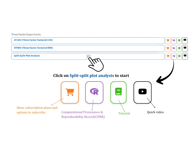
Once the design is understood, the analysis can be performed in RAISINS. Visit the RAISINS home page at www.raisins.live and open the Analysis of experiment section, under Three Factor Experiments. The listing places Split-Split Plot Analysis alongside the two other three-factor designs, 3FCRD and 3FRBD (Figure 2). Click Split-Split Plot Analysis to start.
Each module provides four icons for accessing related resources. The cart shows subscription plans and options, the R icon opens the Computational Provenance & Reproducibility Record described below, the book opens this tutorial, and the play button opens a quick video walkthrough.
3.1 Computational Provenance & Reproducibility Record
CPRR (Computational Provenance & Reproducibility Record) provides a transparent and comprehensive record. Click the CPRR icon shown in Figure 2 to see the exact computational workflow behind the analysis. The record for this module states the R version and the exact version of every package used, and names the specific function behind each reported result. CPRR lists every default parameter and decision rule applied by the module, including how the three error terms are formed and how each critical difference is computed, and provides fully runnable R code that reproduces each analytical step. Users can execute the code in R to independently reproduce and verify the results. It carries its own DOI.
To cite the platform itself in a paper, thesis, or report, use the RAISINS citation, available in APA, Harvard, and BibTeX formats at www.raisins.live/citation.html. That is the primary reference, and for most manuscripts it is all you need.
The CPRR for the split-split-plot module is at www.raisins.live/module_record/splitsplit.html.
Cite the RAISINS paper as your primary reference for the platform. Add the CPRR as supporting documentation when a journal asks for details of the computing environment, or when you want your methods section to be precise about versions and functions rather than saying “analysis was carried out using an online tool.” The CPRR supports the citation and ensures computational reproducibility.
4 Preview mode and Quick Tour
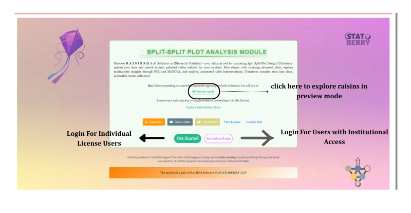
Before subscribing, the complete module can be explored using Preview mode, offered on the module’s Welcome page (Figure 3). Preview mode loads a built-in split-split-plot dataset so that the available features can be examined; data upload is disabled in this mode. The Welcome page also carries Get Started for individual-licence users and Institutional Login for users with institutional access, a Subscribe link, a Quick video walkthrough, and a Quick Tour that steps through the main controls and can be repeated at any time from the Quick Tour tab.
5 A working example
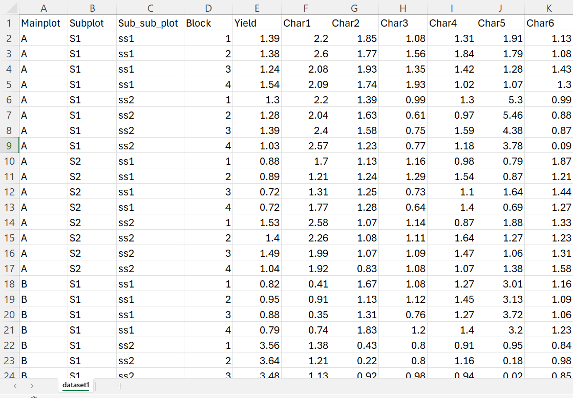
The rest of this tutorial follows one dataset, shown in Figure 5. It is a split-split-plot experiment with Mainplot as factor A at 2 levels (A, B), Subplot as factor B at 2 levels (S1, S2), Sub_sub_plot as factor C at 2 levels (ss1, ss2), and 4 blocks, giving \(2 \times 2 \times 2 \times 4 = 32\) observations, one per row. The layout is exactly the one drawn in Figure 1, repeated four times, once per block, and once more for the second whole-plot level.
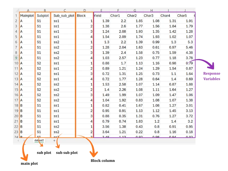
The first four columns hold the whole-plot label, the subplot label, the sub-subplot label and the block number; every remaining column is a response. Seven traits were recorded, Yield and Char1–Char6, though the analysis walked through in this tutorial selects five of them, Yield, Char1, Char2, Char3, Char4, at once. The first row of the file records the sub-subplot that received whole-plot treatment A, subplot treatment S1 and sub-subplot treatment ss1 in block 1, with a Yield of 1.39, a Char1 of 2.2 and a Char2 of 1.85.
This dataset ships with the module as Dataset 1 on the Datasets tab (Section 6.3). If you want to follow the tutorial exactly, download it there and upload it under Analysis.
6 How to prepare your data
The quality of an analysis depends on the quality and structure of the input data. For a split-split-plot analysis, the treatment and replication structure must be represented correctly across all three strata. RAISINS provides four ways to prepare the dataset:
- Create your dataset in MS Excel
- Build your dataset directly within the RAISINS app
- Use the Model datasets in RAISINS as a reference
- Create your dataset using the RA-One chat assistant
6.1 Preparing data in MS Excel
Lay the file out exactly as in Figure 5: the first column holds the whole-plot levels (here Mainplot, with levels A and B), the second column the subplot levels (here Subplot, with levels S1 and S2), the third column the sub-subplot levels (here Sub_sub_plot, with levels ss1 and ss2), the fourth column the block (here Block, numbered 1–4), and each further column is one response variable (Yield, Char1, Char2, …). Every row is one sub-subplot, the smallest unit on which a measurement was taken, so a file for a \(2 \times 2 \times 2 \times 4\) experiment has 32 data rows beneath the header.
Two rules are particularly important. First, keep each treatment label consistent throughout the dataset, for example, use A rather than alternating between A, a, and A. Second, ensure that every sub-subplot treatment appears once within every whole-plot × subplot × block combination, and that every subplot treatment appears once within every whole-plot × block combination. This complete nesting at both levels is required to represent the split-split-plot structure and to estimate all three error terms correctly. Avoid blank rows within the dataset and save the completed file as CSV before uploading.
Dataset creation rules
- Column naming convention
- No spaces allowed in column names.
- Use underscores (
_) or full stops (.) for separation. - Avoid symbols and special characters such as %, #.
- Data arrangement
- Start the data towards the upper-left corner.
- Ensure the row above the data is not blank.
- Cell management
- Avoid typing or deleting in cells without data.
- If needed, select the affected cells, right-click, and choose Clear Contents.
- Main Plot, Sub Plot, Sub-sub Plot, Block and response columns
- The first four columns must be the whole-plot factor, the subplot factor, the sub-subplot factor and the block; every remaining column is a numeric response.
- Use the same label for a level everywhere it appears, so RAISINS reads the correct number of levels and replications at every stratum.
- The nesting must be complete at both levels
- Each whole-plot treatment appears once per block, each subplot treatment appears once inside each of those whole plots, and each sub-subplot treatment appears once inside each of those subplots. Do not average sub-subplots into a single row, and do not omit a treatment combination from a block; the design must stay balanced for the standard errors and critical differences to be exact.
How to save as CSV in MS Excel
Open your workbook. Ensure your data is arranged properly with only one sheet.
Click the ‘File’ menu. Go to the top-left corner and click File.
Choose ‘Save As’ or ‘Save a Copy’. Select the location where you want to save your file.
Set file type to CSV. In the ‘Save as type’ dropdown, choose CSV (Comma delimited) (*.csv).
Name your file. Enter a relevant file name without spaces (use underscores if needed).
Click ‘Save’. Click Save to export the file.
💡 Tip: Before saving, double-check that your data is on the first sheet and follows the required format.
6.2 Prepare using Create Data in RAISINS
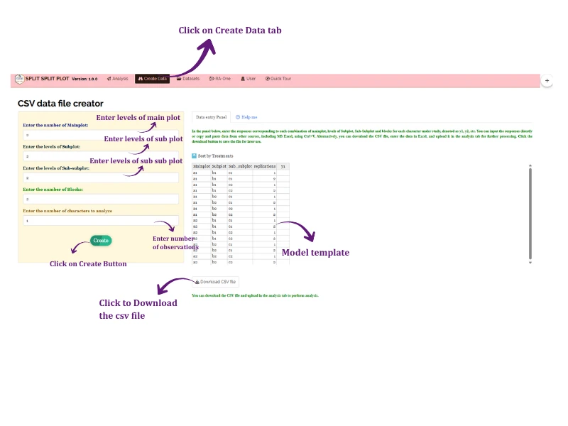
If you are unsure about the correct format, RAISINS can build the layout for you. Open the Create Data tab and fill in five boxes (Figure 6):
- Enter the levels of Mainplot - how many levels the whole-plot factor has,
- Enter the levels of Subplot - how many levels the subplot factor has,
- Enter the levels of Sub-subplot - how many levels the sub-subplot factor has,
- Enter the number of Blocks - how many times the whole layout is repeated,
- Enter the number of characters to analyze - how many response variables you plan to measure.
Click Create. The Data entry Panel generates one row for each whole-plot × subplot × sub-subplot × block combination and provides empty response columns (y1, y2, …) for data entry. Values can be entered manually or pasted from Excel using Ctrl + V. The Sort by Treatments option groups related treatment combinations together for convenient data entry; the order of rows does not affect the analysis. After completing the table, click Download CSV file and upload the file under the Analysis tab.
6.3 Download the Model datasets
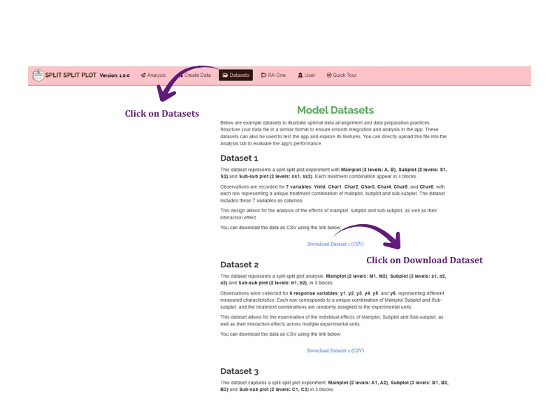
If you would like to explore the module before using your own data, RAISINS provides model datasets on the Datasets tab (Figure 7), each described in full before you download it. Dataset 1 is the file used throughout this tutorial: Mainplot at 2 levels (A, B), Subplot at 2 levels (S1, S2), Sub-sub plot at 2 levels (ss1, ss2), each combination appearing in 4 blocks, with 7 response variables, Yield and Char1–Char6. Dataset 2 represents Mainplot at 2 levels (M1, M2), Subplot at 3 levels (a1, a2, a3) and Sub-sub plot at 2 levels (b1, b2) in 3 blocks, with 6 response variables y1–y6. Dataset 3 captures Mainplot at 2 levels (A1, A2), Subplot at 3 levels (B1, B2, B3) and Sub-sub plot at 2 levels (C1, C2), also in 3 blocks. To use one:
- Open the Datasets tab
- Read the description and click the Download Dataset (CSV) link beneath it
- Save the file, then either study its layout as a reference for your own file or upload it directly under Analysis to see the full analysis at once
6.4 Creating a dataset using RA-One chat
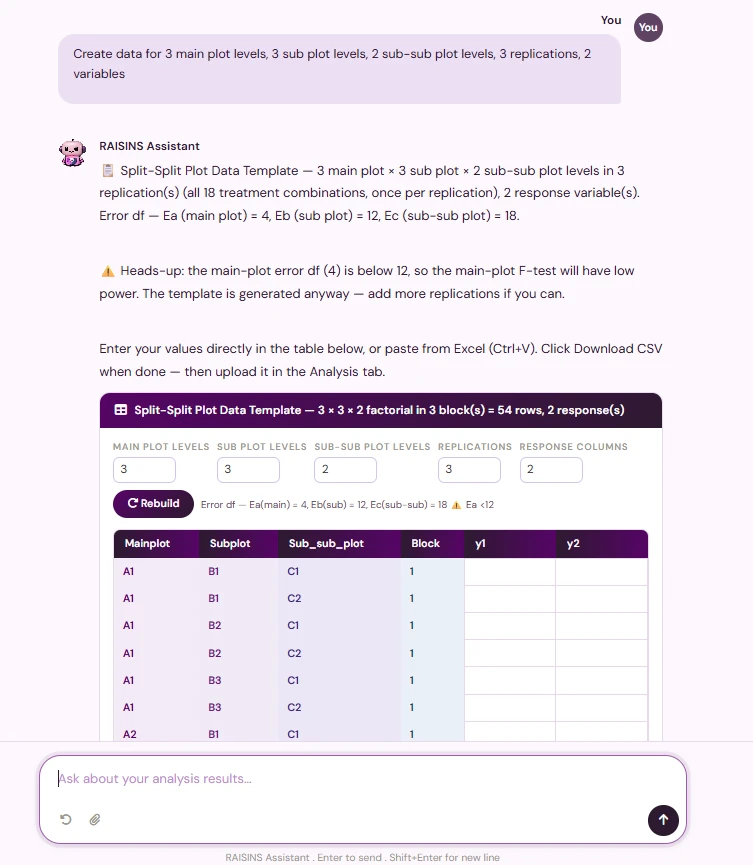
RA-One, the built-in chat assistant, can build a correctly formatted template through an ordinary conversation. Open the RA-One tab and describe your experiment in plain language, for instance “Create data for 3 main plot levels, 3 sub plot levels, 2 sub-sub plot levels, 3 replications, 2 variables” (Figure 8). RA-One returns a ready-to-fill template, here a 3 × 3 × 2 factorial in 3 blocks = 54 rows, 2 response(s), with the Mainplot, Subplot and Sub_sub_plot columns already filled in, the requested number of blocks, and empty y1, y2 columns for your readings.
RA-One does something the plain template cannot: it checks the size of the design for you. Above the table it prints the error degrees of freedom for all three strata, here Ea(main) = 4, Eb(sub) = 12, Ec(sub-sub) = 18, together with a warning icon whenever a stratum’s error df falls below the conventional threshold of 12, in this example Ea <12, flagging that the whole-plot test will have low power. If the design looks too thin, change the level counts in the boxes provided and click Rebuild before you ever collect data. Fill in the responses, download the CSV, and upload it under Analysis.
All three in-app routes ask for exactly the same four numbers, levels of the whole-plot factor, levels of the subplot factor, levels of the sub-subplot factor, and number of blocks, and produce \(a \times b \times c \times r\) rows. The template directly represents the required observation count: one row per sub-subplot, with all three error-df formulas printed back to you.
7 The Analysis tab
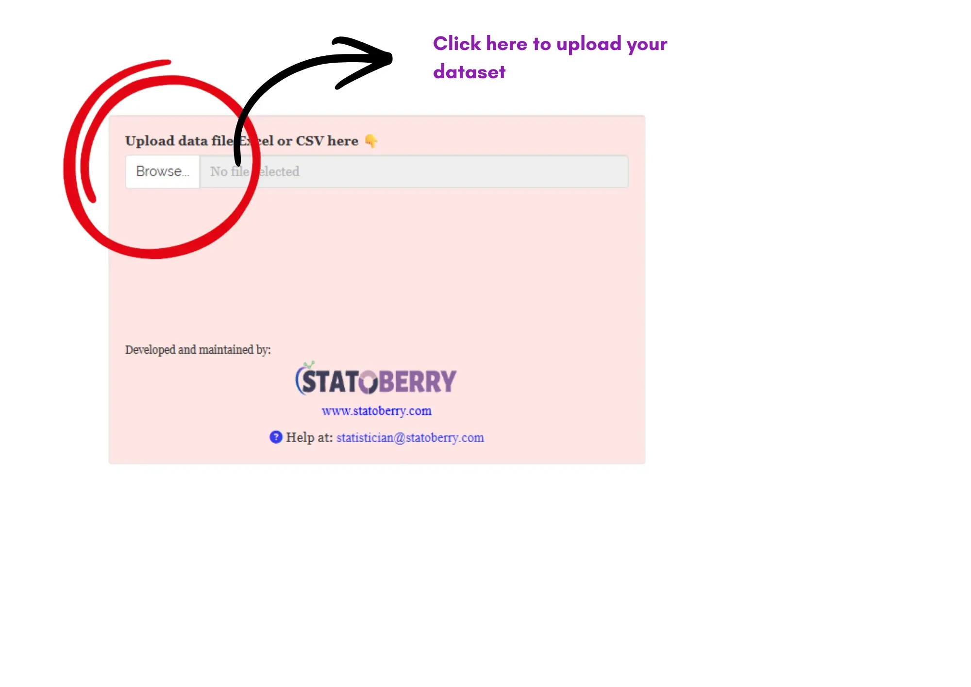
After preparing the CSV file, open the Analysis tab. Click Browse… under Upload data file Excel or CSV here and select the CSV file (Figure 9). A blue Upload complete message confirms that the file has been loaded.
Once the file is in, RAISINS reads its column names and asks you to point it at the right columns (Figure 10). The selectors follow the structure of the design exactly, from the largest unit to the smallest:
- Select Main Plot - the column holding the whole-plot levels; here
Mainplot, with levels A and B. - Select Sub Plot - the column holding the subplot levels; here
Subplot, with levels S1 and S2. - Select sub-sub Plot - the column holding the sub-subplot levels; here
Sub_sub_plot, with levels ss1 and ss2. - Select the blocks - the column identifying the block; here
Block, numbered 1 to 4. - Select variables - one or more response columns to analyse. You may select several at once, here
Yield, Char1, Char2, Char3, Char4, and RAISINS analyses each in turn. - Click for Transformation - an optional toggle to transform a skewed response before analysis.
Getting these three selectors the right way round matters more here than in any other module, because there are three of them. The whole-plot, subplot and sub-subplot columns are not interchangeable: they decide which factor is tested against Error(a), which against Error(b), and which against Error(c), and therefore how much precision each factor receives. If you swap any two, the analysis will still run and still produce a table, but it will be answering a different experiment from the one you carried out.
When the columns are chosen, click Run Analysis!. RAISINS fits the split-split-plot model to every selected response and fills the results sub-tabs, Analysis Results, Summary stats, Individual ANOVA, Basic Plots, Advanced Plots, Interpretation, Multivariate, FAQs and View Data.
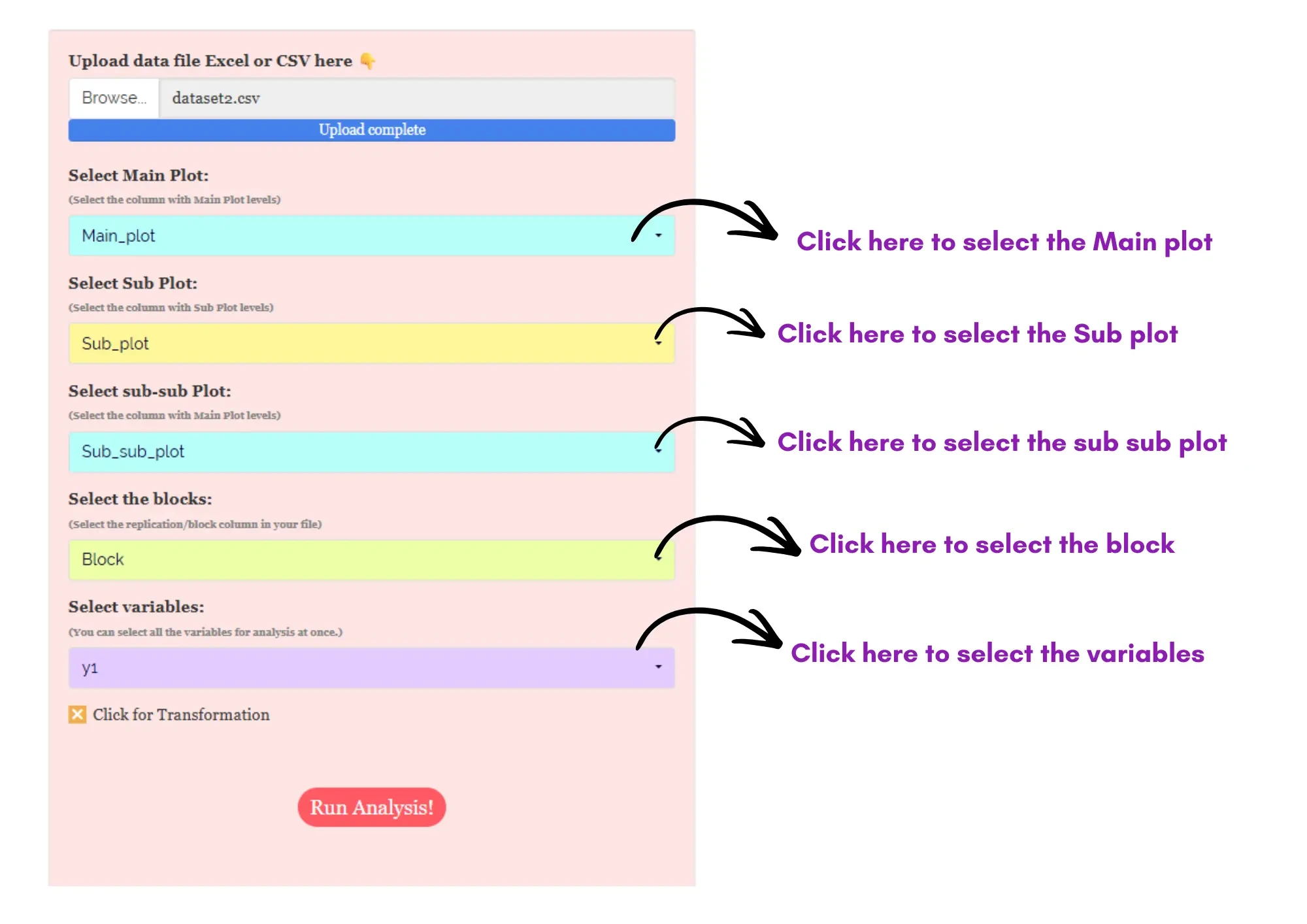
You do not need to run the module once per response. Select several response columns together and RAISINS produces a complete ANOVA, mean-comparison and effect-size table for each. This is why every results table in the next section carries one column per trait, Yield through Char4.
7.1 Optional: transforming a response
The split-split-plot ANOVA assumes that the model residuals are approximately normally distributed and that the variability is reasonably similar across treatment combinations. If a response is strongly skewed or its variability increases with its mean, select Click for Transformation before running the analysis and choose an appropriate transformation. RAISINS then performs the analysis on the transformed scale and reports the transformed mean in parentheses alongside the original mean, allowing the analysis to be traced clearly.
A transformation is a temporary change of scale to make the test valid; it does not change your experiment. Report that a transformation was used, but discuss the means and recommendations in the original units. If no assumption is violated, leave the toggle off, an unnecessary transformation only makes the results harder to read.
8 Analysis results
The Analysis Results sub-tab presents the split-split-plot ANOVA results. The control strip lets you select the multiple-comparison test (LSD by default), the level of significance (\(\alpha\), 0.05 by default), the number of digits after decimal, and the font (Figure 11). RAISINS also prints a plain-language summary of the design and analysis settings: “This study is a Split-Split design with 4 blocks. The data includes Mainplot (denoted as Mainplot) with 2 levels (A & B), Subplot (denoted as Subplot) with 2 levels (S1 & S2) and Sub_sub_plot (denoted as Sub-subplot) with 2 levels (ss1 & ss2). A total of 8 treatment combinations were evaluated, each replicated 4 times. You have selected Least Significant Difference (LSD) (post-hoc test) for pairwise comparisons at a 0.05 level of significance.”
Below that summary sit the result tables: the ANOVA summary, then the whole-plot, subplot and sub-subplot means, then every interaction. Each table contains a separate column for each response variable.
The note concerning critical differences is important: CD values are calculated only if ANOVA detects a significant difference. If ANOVA is not significant, no CD is calculated, and a ‘-’ is shown. Therefore, a dash in a CD row indicates that the corresponding ANOVA test was not significant; it does not indicate missing data.
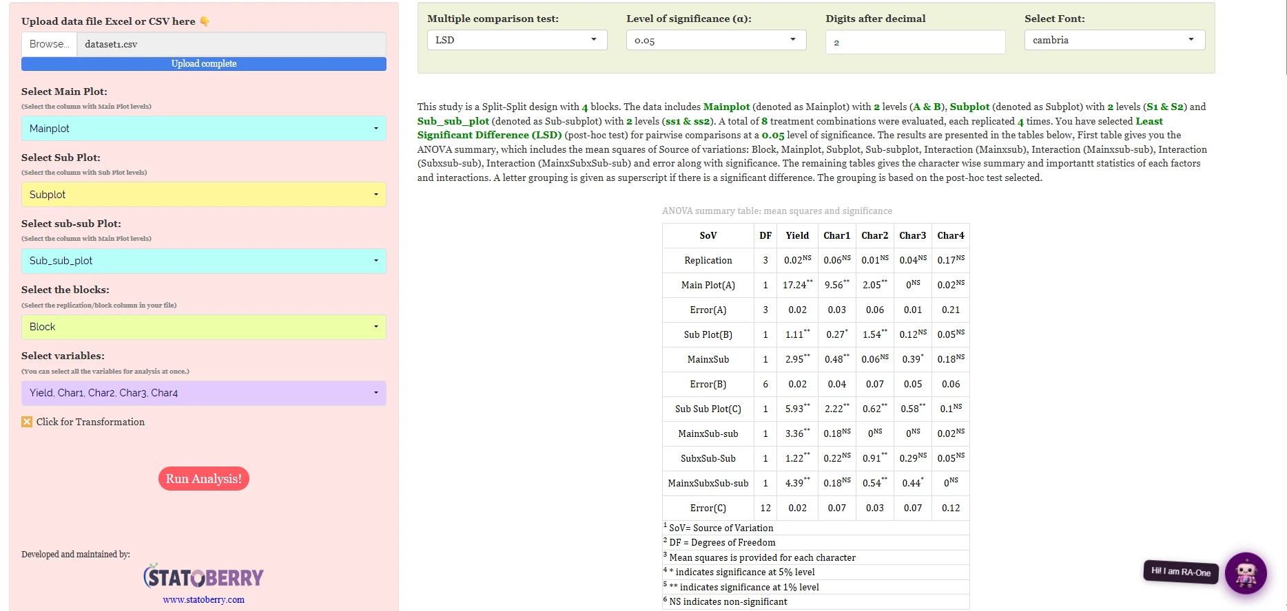
Table 1: ANOVA summary - mean squares and significance
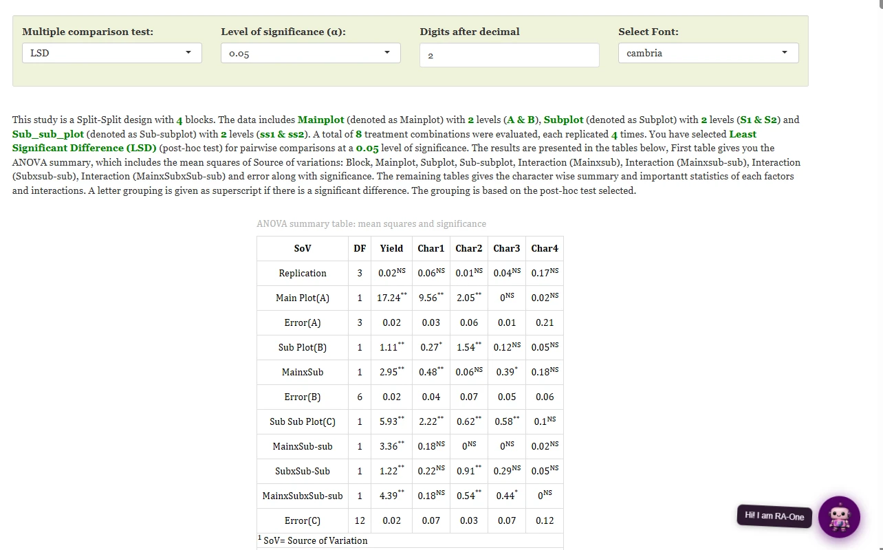
This table reflects the three strata described in Section 2. Its row order shows how the sources of variation are separated in a split-split-plot design. Replication (3 df) comes first, then Main Plot(A) (1 df) and immediately beneath it Error(A) (3 df), the error against which the whole-plot factor is tested. Next comes the middle storey: Sub Plot(B) (1 df), MainxSub (1 df) and Error(B) (6 df), the error against which both are tested. Finally the finest storey: Sub Sub Plot(C) (1 df), MainxSub-sub (1 df), SubxSub-Sub (1 df), MainxSubxSub-sub (1 df) and Error(C) (12 df), the error against which all four of those sources are tested. The degrees of freedom match the formulas in Section 2 exactly for a \(2 \times 2 \times 2 \times 4\) experiment.
Each cell is that source’s mean square for the response, carrying a superscript flag: * for significance at 5%, ** at 1%, and NS for non-significant. Scanning the table shows a design in which the whole-plot factor and the sub-subplot factor dominate. Main Plot(A) is significant at 1% for Yield (\(17.24^{**}\)) and Char1 (\(9.56^{**}\)), and at 1% for Char2 too (\(2.05^{**}\)), but non-significant for Char3 and Char4. Sub Sub Plot(C) is significant for four of the five traits, Yield (\(5.93^{**}\)), Char1 (\(2.22^{**}\)), Char2 (\(0.62^{**}\)) and Char3 (\(0.58^{**}\)), non-significant only for Char4. Every one of the four interaction rows, MainxSub, MainxSub-sub, SubxSub-Sub and MainxSubxSub-sub, is significant for Yield at the 1% level, and several are significant for the other traits as well, Char1 for MainxSub (\(0.48^{**}\)), Char2 for SubxSub-Sub (\(0.91^{**}\)) and MainxSubxSub-sub (\(0.54^{**}\)), and Char3 for MainxSub (\(0.39^{*}\)) and MainxSubxSub-sub (\(0.44^{*}\)). Char4 is the exception throughout the table, non-significant for every treatment source, whole-plot, subplot, sub-subplot and every interaction alike.
In a one-stratum ANOVA there is a single Error row, and every treatment mean square is divided by it. Here there are three, and each one belongs to a particular stratum. Error(A) measures how much whole plots that received the same whole-plot treatment differ from one another, so it is the right denominator for the Main Plot(A) test and nothing else. Error(B) measures how much subplots within the same whole plot differ, so it is the right denominator for Sub Plot(B) and for A × B. Error(C) measures how much sub-subplots within the same subplot differ, so it is the right denominator for Sub-Sub Plot(C) and for every interaction that involves C, A × C, B × C, and A × B × C. Using a single pooled error anywhere in this table would test some sources too generously and others too harshly. The whole design exists to keep these three strata apart.
How this table is built
RAISINS fits the split-split-plot linear model for each trait, with the replication effect, the whole-plot effect and the whole-plot error forming the top stratum, the subplot effect, the A × B interaction and the subplot error forming the middle stratum, and the sub-subplot effect together with A × C, B × C, A × B × C and the sub-subplot error forming the bottom stratum. Each source’s mean square is its sum of squares divided by its degrees of freedom. The F-test for Main Plot(A) divides its mean square by Error(A); the F-tests for Sub Plot(B) and A × B divide theirs by Error(B); the F-tests for Sub-Sub Plot(C), A × C, B × C and A × B × C all divide theirs by Error(C). The p-value behind each F decides the * / ** / NS flag against the chosen \(\alpha\). The CPRR (Section 3.1) names the exact function used and prints runnable R code for each step.
Table 2: Main Plot (A) - means and comparison statistics
| Yield | Char1 | Char2 | Char3 | Char4 | |
|---|---|---|---|---|---|
| A | 1.20±0.28 | 2.06±0.41 | 1.38±0.33 | 1.08±0.35 | 1.29±0.28 |
| B | 2.67±1.10 | 0.96±0.40 | 0.87±0.45 | 1.10±0.29 | 1.34±0.38 |
| F stat | 716.13** | 299.56** | 35.98** | 0.40 NS | 0.08 NS |
| p value | 0.00 | 0.00 | 0.01 | 0.57 | 0.80 |
| CD (A) | 0.17 | 0.20 | 0.27 | - | - |
| MSE(A) | 0.02 | 0.03 | 0.06 | 0.01 | 0.21 |
| SE(m) | 0.04 | 0.04 | 0.06 | 0.03 | 0.12 |
| SE(d) | 0.05 | 0.06 | 0.08 | 0.04 | 0.16 |
| CV(%) | 8.02 | 11.82 | 21.16 | 9.27 | 34.96 |
The whole-plot table presents the means for the two levels of the whole-plot factor, averaged over subplot and sub-subplot treatments and blocks. Three of the five traits separate cleanly: Yield is \(2.67 \pm 1.10\) for B against \(1.20 \pm 0.28\) for A, a gap far in excess of \(CD(A) = 0.17\); Char1 runs the other way, \(2.06 \pm 0.41\) for A against \(0.96 \pm 0.40\) for B, against \(CD(A) = 0.20\); and Char2 is higher under A (\(1.38 \pm 0.33\)) than B (\(0.87 \pm 0.45\)), against \(CD(A) = 0.27\). Char3 and Char4 show no significant whole-plot effect, so their CD (A) entries read “–”. Note also how few degrees of freedom this test rests on, \(F\) is evaluated against Error(A) at only 3 df (Figure 12), which is why a whole-plot effect has to be large, as these three clearly are, before it registers as significant at all.
Table 3: Sub Plot (B) - means and comparison statistics
| Yield | Char1 | Char2 | Char3 | Char4 | |
|---|---|---|---|---|---|
| S1 | 1.75±1.07 | 1.60±0.76 | 1.35±0.51 | 1.03±0.35 | 1.28±0.25 |
| S2 | 2.12±1.11 | 1.42±0.61 | 0.91±0.28 | 1.15±0.27 | 1.36±0.40 |
| F stat | 45.48** | 6.99* | 22.07** | 2.29 NS | 0.85 NS |
| p value | 0.00 | 0.04 | 0.00 | 0.18 | 0.39 |
| CD (B) | 0.13 | 0.17 | 0.23 | - | - |
| MSE(B) | 0.02 | 0.04 | 0.07 | 0.05 | 0.06 |
| SE(m) | 0.04 | 0.05 | 0.07 | 0.06 | 0.06 |
| SE(d) | 0.06 | 0.07 | 0.09 | 0.08 | 0.09 |
| CV(%) | 8.06 | 13.05 | 23.42 | 20.79 | 18.51 |
The subplot table has the identical layout, now averaging over the whole plots and sub-subplots to show the effect of the subplot factor across its two levels, S1 and S2, with CD (B) as its critical difference and Error(B) at 6 df behind the F-test. Yield (\(2.12 \pm 1.11\) for S2 against \(1.75 \pm 1.07\) for S1), Char1 (\(1.60 \pm 0.76\) for S1 against \(1.42 \pm 0.61\) for S2) and Char2 (\(1.35 \pm 0.51\) for S1 against \(0.91 \pm 0.28\) for S2) all separate at 1% or 5%, while Char3 and Char4 are non-significant and their CD (B) rows read “–”.
Table 4: Sub-Sub Plot (C) - means and comparison statistics
| Yield | Char1 | Char2 | Char3 | Char4 | |
|---|---|---|---|---|---|
| ss1 | 1.50±0.91 | 1.25±0.73 | 1.27±0.52 | 1.23±0.36 | 1.37±0.38 |
| ss2 | 2.37±1.11 | 1.77±0.53 | 0.99±0.37 | 0.96±0.19 | 1.26±0.27 |
| F stat | 304.63** | 30.02** | 21.46** | 8.85** | 0.78 NS |
| p value | 0.00 | 0.00 | 0.00 | 0.01 | 0.39 |
| CD (C) | 0.11 | 0.21 | 0.13 | 0.20 | - |
| MSE(C) | 0.02 | 0.07 | 0.03 | 0.07 | 0.12 |
| SE(m) | 0.03 | 0.07 | 0.04 | 0.06 | 0.09 |
| SE(d) | 0.05 | 0.10 | 0.06 | 0.09 | 0.12 |
| CV(%) | 7.21 | 18.00 | 15.14 | 23.41 | 26.56 |
The sub-subplot table averages over the whole plots and subplots to show the effect of the sub-subplot factor across ss1 and ss2, with CD (C) as its critical difference and Error(C), the largest error term at 12 df, behind the F-test. Four of the five traits separate significantly here, Yield, Char1, Char2 and Char3 all favour ss2, and only Char4 fails to reach significance. Because Error(C) carries four times the degrees of freedom of Error(A), the sub-subplot test is comfortably the most powerful of the three single-factor tests in this experiment, which is exactly the trade-off Section 1 describes: the easiest-to-change factor is estimated with the greatest precision.
Table 5: Interaction Main x Sub plot (A × B) - cell means and comparison statistics
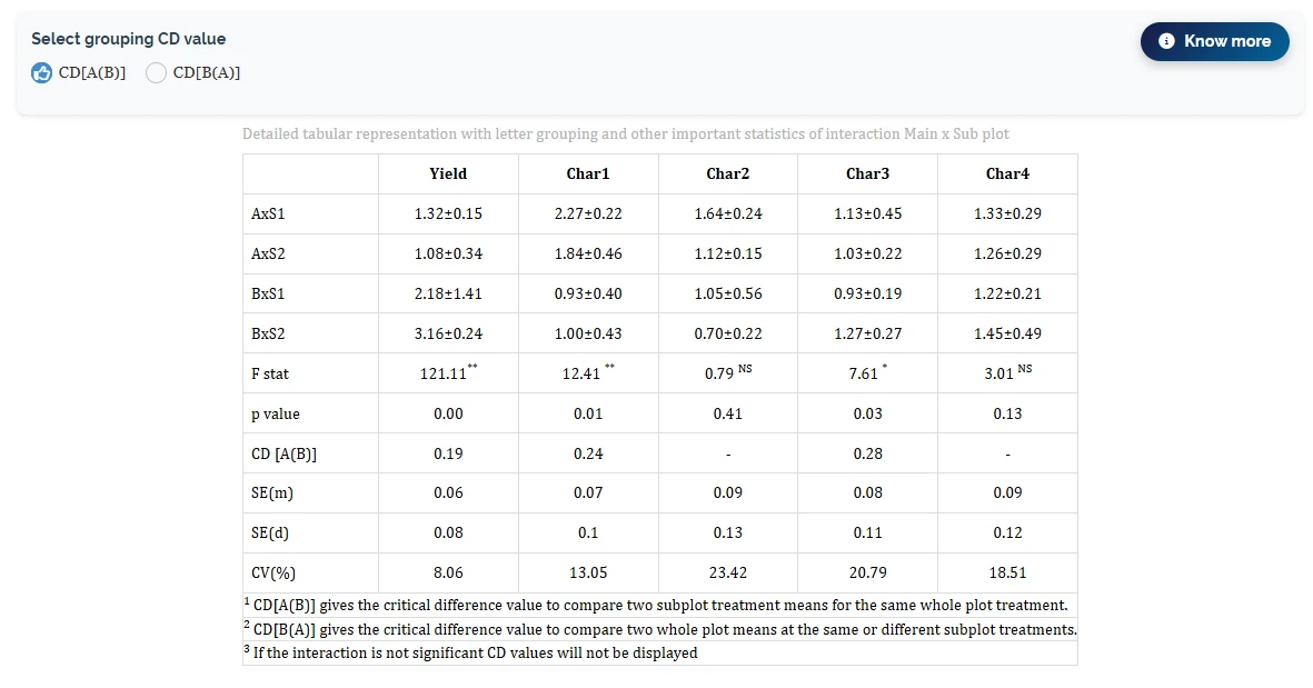
The A × B interaction is significant for three of the five traits: Yield (\(F = 121.11^{**}\), \(p = 0.00\)), Char1 (\(F = 12.41^{**}\), \(p = 0.01\)) and Char3 (\(F = 7.61^{*}\), \(p = 0.03\)); Char2 and Char4 are non-significant, and their CD rows read “–”. With the selector set to CD[A(B)], the printed critical differences are 0.19 for Yield, 0.24 for Char1 and 0.28 for Char3. For Yield the four cells are AxS1 \(1.32 \pm 0.15\), AxS2 \(1.08 \pm 0.34\), BxS1 \(2.18 \pm 1.41\) and BxS2 \(3.16 \pm 0.24\), so the largest gap sits between BxS2 and AxS2, a difference of 2.08 against a critical difference of only 0.19. For Char1 the pattern reverses, AxS1 (\(2.27 \pm 0.22\)) and AxS2 (\(1.84 \pm 0.46\)) sit well above the two B rows.
Table 6: Interaction Main x Sub-sub plot (A × C) - cell means and comparison statistics
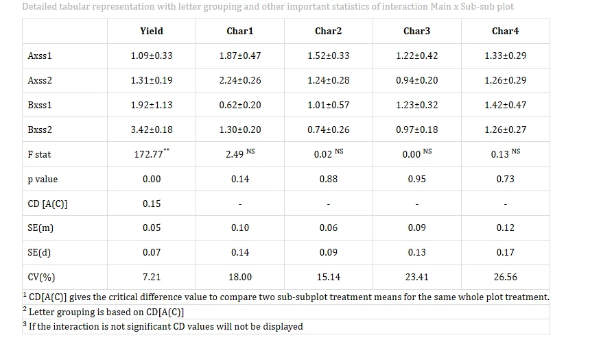
Only Yield shows a significant A × C interaction here, \(F = 172.77^{**}\), \(p = 0.00\), against \(CD[A(C)] = 0.15\). The four cells are Axss1 \(1.09 \pm 0.33\), Axss2 \(1.31 \pm 0.19\), Bxss1 \(1.92 \pm 1.13\) and Bxss2 \(3.42 \pm 0.18\), so Bxss2 stands well clear of every other combination. Char1 through Char4 are all non-significant for this interaction, so their CD rows read “–”. Notice that this table offers only the CD[A(C)] direction, comparing sub-subplot means within the same whole plot, unlike the A × B table, which lets you switch between both directions; the definitions themselves, and how a “compare-within” CD differs from a “compare-across” CD, are set out fully in Section 8.1.
RAISINS also fits and tests the B × C interaction, and its mean square appears as the SubxSub-Sub row of Figure 12, significant for Yield (\(1.22^{**}\)) and Char2 (\(0.91^{**}\)), non-significant for Char1, Char3 and Char4. A screenshot of the dedicated B × C cell-means table, with its own CD[B(C)] / CD[C(B)] selector, was not available for this tutorial and is not shown here.
The reasoning is identical to the A × B table above, only one stratum down: CD[B(C)] compares sub-subplot means within the same subplot, using Error(C); CD[C(B)] compares subplot means across sub-subplot treatments, and therefore mixes Error(B) and Error(C). Both are defined precisely in Section 8.1.
Table 7: Interaction Main x Sub x Sub-sub plot (A × B × C) - cell means and comparison statistics
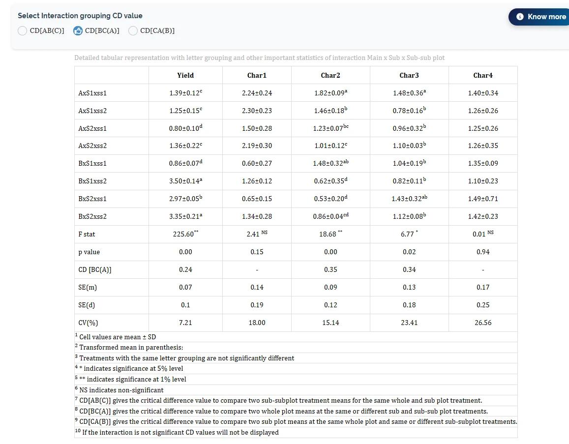
This is the table the split-split-plot design was built to produce. Its rows are the eight treatment combinations, every whole-plot level crossed with every subplot level crossed with every sub-subplot level. The three-way interaction is significant for Yield (\(F = 225.60^{**}\), \(p = 0.00\)), Char2 (\(F = 18.68^{**}\), \(p = 0.00\)) and Char3 (\(F = 6.77^{*}\), \(p = 0.02\)); Char1 and Char4 are non-significant. With the selector set to CD[BC(A)], the printed critical difference for Yield is 0.24. Reading the letters, BxS1xss2 (\(3.50 \pm 0.14\)) and BxS2xss2 (\(3.35 \pm 0.21\)) share letter a and stand apart from AxS2xss1 (\(0.80 \pm 0.10\), letter d) and BxS1xss1 (\(0.86 \pm 0.07\), also letter d), the lowest pair, while BxS2xss1 (\(2.97 \pm 0.05\), letter b) sits between them. For Char2, AxS1xss1 (\(1.82 \pm 0.09\), letter a) is highest and BxS1xss2 (\(0.62 \pm 0.35\)) and BxS2xss1 (\(0.53 \pm 0.20\)), both letter d, are lowest.
The lower rows report the standard error of a mean SE(m), the standard error of a difference SE(d) and the coefficient of variation CV(%). Because this is the finest stratum, these are the same SE(m)/SE(d)/CV(%) figures already seen in Table 4: 7.21% for Yield up to 26.56% for Char4, which tells you Char4 was measured with far less precision than Yield, and would need a much larger effect before any test could detect it.
8.1 The critical differences of a split-split-plot
A split-split-plot needs more than one critical difference because it needs more than one error term, and RAISINS names each CD after the comparison it serves. Above the interaction tables, RAISINS provides radio-button selectors, CD[A(B)] and CD[B(A)] above the A × B table, CD[B(C)] and CD[C(B)] above the B × C table, and CD[AB(C)], CD[BC(A)] and CD[CA(B)] above the three-way table, together with a Know more button that repeats these definitions on demand.
The reason for this proliferation follows directly from the nested layout in Figure 1. Some comparisons stay inside a single subplot or a single whole plot, and some have to cross from one to another. Those two kinds of comparison do not carry the same amount of noise, so they cannot share one yardstick. RAISINS states the definitions in the footnotes of the interaction tables, in these words:
| Critical difference | What it compares |
|---|---|
| CD[A(B)] | “the critical difference value to compare two subplot treatment means for the same whole plot treatment” |
| CD[B(A)] | “the critical difference value to compare two whole plot means at the same or different subplot treatments” |
| CD[B(C)] | “the critical difference value to compare two sub-subplot treatment means for the same sub plot treatment” |
| CD[C(B)] | “the critical difference value to compare two sub plot means at the same or different sub-subplot treatments” |
| CD[AB(C)] | “the critical difference value to compare two sub-subplot treatment means for the same whole and sub plot treatment” |
| CD[BC(A)] | “the critical difference value to compare two whole plot means at the same or different sub and sub-sub plot treatments” |
| CD[CA(B)] | “the critical difference value to compare two sub plot means at the same whole plot and same or different sub-subplot treatments” |
Put in the terms of the working example: comparing subplot S1 with S2 within whole plot A is a CD[A(B)] comparison, because both subplots sit inside the same whole plot and differ only in the subplot treatment itself, so the comparison rests on Error(B) alone. Comparing AxS1 with BxS1 is a CD[B(A)] comparison, because the two subplots being compared lie in different whole plots, so any difference between them carries whole-plot noise (Error(A)) on top of subplot noise (Error(B)). The same logic drops one storey for CD[B(C)] and CD[C(B)]: comparing ss1 with ss2 within the same subplot is a CD[B(C)] comparison, resting on Error(C) alone, while comparing a subplot mean at one sub-subplot treatment against the same or a different sub-subplot treatment is a CD[C(B)] comparison, and mixes Error(B) with Error(C).
The three-way selector works the same way, one stratum further out. CD[AB(C)] compares sub-subplot means while both the whole plot and the subplot are held fixed, so it rests on Error(C) alone, and is the CD the letter groupings in Figure 15 are ordinarily based on. CD[BC(A)], the option selected in Figure 15, compares whole-plot means while subplot and sub-subplot treatments are allowed to be the same or different, so it is built from all three error terms and is the most conservative of the three. CD[CA(B)] sits between the two, comparing subplot means at a fixed whole plot but a same-or-different sub-subplot treatment, mixing Error(B) and Error(C).
Consequently, a CD that lets more strata vary between the two things being compared is always the larger, more conservative yardstick. Comparisons that stay entirely within the finest stratum, sub-subplot treatments within the same subplot, are detected most easily; comparisons that cross the coarsest stratum, whole-plot means, are the hardest to separate. This ordering of precision is an inherent feature of the split-split-plot design, not a quirk of this particular dataset.
Every interaction table in this module carries its own footnote defining exactly which comparison its printed CD serves, and, for the A × B and three-way tables, a radio button that changes which CD (and which letters) are shown. Before writing “combination X differs significantly from combination Y” in a report, check which button was selected and which definition applies, comparisons that cross a stratum boundary need the wider, cross-stratum CD, not the narrower within-stratum one that happens to be on screen.
The arithmetic behind the yardsticks
Every critical difference in this module has the same shape, a \(t\) value multiplied by the standard error of a difference, \(CD = t \times SE(d)\); what differs is which error mean squares enter the standard error and how many degrees of freedom the \(t\) carries.
For a comparison that stays inside one stratum, two sub-subplot means at the same whole plot and subplot (CD[A(B)]-style, or CD[AB(C)] in the three-way table), the standard error is built from \(MSE_c\) alone, with \(t\) based on the Error(c) degrees of freedom (12 in the working example). This is the most precise, and therefore smallest, of the family.
For a comparison that crosses exactly one boundary, two subplot means at the same whole plot but different sub-subplot treatments (CD[C(B)] or CD[CA(B)]), the standard error mixes \(MSE_b\) and \(MSE_c\), and the appropriate \(t\) is a weighted blend of the \(t\) values for Error(b) and Error(c) rather than a single tabulated value.
For a comparison that crosses two boundaries, two whole-plot means at the same or different subplot and sub-subplot treatments (CD[B(A)], CD[BC(A)]), the standard error mixes all three mean squares, \(MSE_a\), \(MSE_b\) and \(MSE_c\), and is therefore the widest and most conservative yardstick in the table. The CPRR for the module (Section 3.1) prints the exact expressions RAISINS evaluates for each of the seven CDs, together with runnable R code, if you need to reproduce or cite them.
8.2 Interpretation from Figure 12
Taken together, the results describe an experiment in which the whole-plot factor and the sub-subplot factor both matter strongly, the subplot factor matters for some traits, and the three factors interact for Yield, Char2 and Char3.
Yield is the clearest story in the dataset: every single source in Figure 12 is significant at the 1% level, whole plot, subplot, sub-subplot, and all four interactions. The three-way cell means in Figure 15 show why, the four B-level combinations sit well above the four A-level combinations, with BxS1xss2 (\(3.50 \pm 0.14\)) the single highest cell and AxS2xss1 (\(0.80 \pm 0.10\)) the lowest, a spread that swamps every critical difference in the table.
Char1 is significant for the whole plot (\(F = 9.56^{**}\)) and the subplot (\(F = 6.99^{*}\)) and sub-subplot (\(F = 30.02^{**}\)) main effects, and for the A × B interaction (\(F = 12.41^{**}\) in Figure 13), but not for any interaction that involves C. Because the three-way and B × C interactions are non-significant for Char1, the correct summary for this trait leans on the whole-plot, subplot and sub-subplot means (Tables 2–4) and the A × B cell means, not the eight-cell breakdown.
Char2 and Char3 both show significant three-way interactions (\(F = 18.68^{**}\) and \(F = 6.77^{*}\) respectively), which means the effect of one factor on these two traits genuinely depends on the levels of the other two. For these traits the eight-cell table in Figure 15, not the single-factor margins, is what should be reported.
Char4 is the exception throughout: every source in Figure 12 is non-significant for this trait. The experiment did not provide sufficient evidence of a whole-plot, subplot, sub-subplot, or interaction effect on Char4 at \(\alpha = 0.05\), and that null result belongs in the report alongside the significant findings for the other four traits, not omitted from it.
A source can be statistically significant on a small mean-square gap once its error term has few degrees of freedom behind it, and can fail to reach significance despite a sizeable mean-square gap when its error term is noisy. Compare the F-statistics in Figure 12 against the CV(%) rows in Tables 2–7 before deciding how much weight a result deserves: a large CV alongside a non-significant F, as with Char4 throughout, is a caution about precision, not necessarily proof that the treatments had no effect.
Reading every row of the results tables
- Mean ± SD - the treatment or cell mean and its standard deviation; a transformed mean, if a transformation was applied, is shown in parentheses.
- F stat / p value - the F-test for that source and its probability; the superscript (
*,**,NS) marks significance at the chosen \(\alpha\). Remember which error each F used: Error(A) for the whole plot, Error(B) for the subplot and A × B, Error(C) for the sub-subplot and every interaction that involves it. - CD (A) / CD (B) / CD (C) - the single-factor critical differences from the selected post-hoc test; two means differing by more than the CD are significantly different. Shown as “–” whenever the corresponding F-test was non-significant.
- CD[A(B)] / CD[B(A)] / CD[B(C)] / CD[C(B)] / CD[AB(C)] / CD[BC(A)] / CD[CA(B)] - the seven nested critical differences explained in Section 8.1.
- SE(m) / SE(d) - standard error of a single mean and of a difference between two means.
- MSE(A) / MSE(B) / MSE(C) - the error mean square for that stratum, i.e. Error(a), Error(b) or Error(c) from Figure 12.
- CV(%) - coefficient of variation, the error SD as a percentage of the grand mean; it gauges experimental precision, and a large value warns that only large effects will be detectable.
9 Summary stats and Individual ANOVA
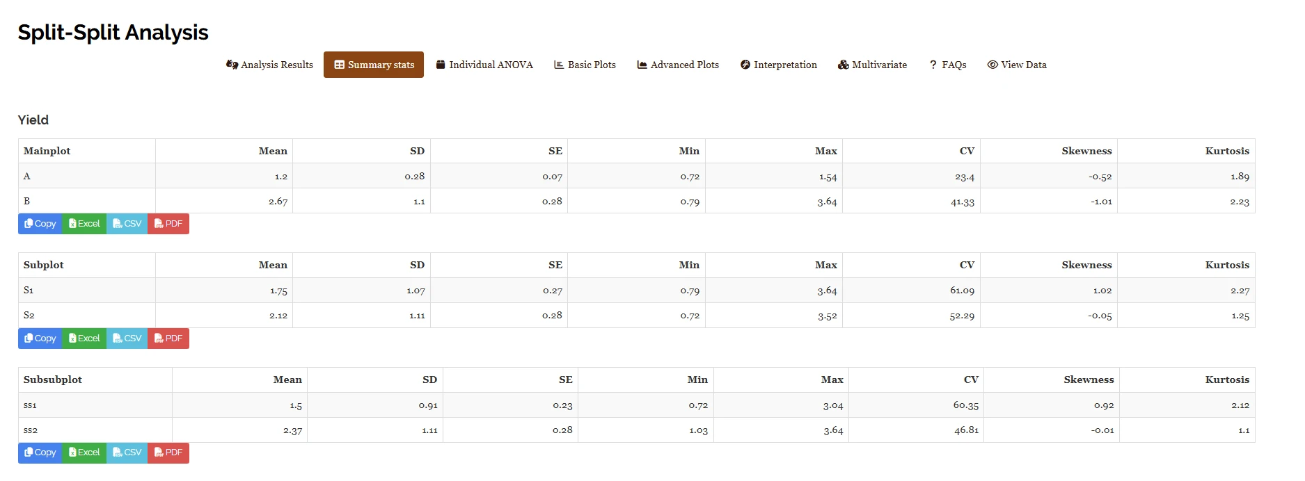
The Summary stats sub-tab (Figure 16) reports descriptive statistics for every response, broken down by each factor in turn, Mainplot, Subplot and Subsubplot. For Yield, the Mainplot breakdown shows A with a mean of 1.20 (SD 0.28, CV 23.4%, skewness \(-0.52\)) against B with a mean of 2.67 (SD 1.10, CV 41.33%, skewness \(-1.01\)); the Subplot breakdown shows S1 at 1.75 against S2 at 2.12; and the Subsubplot breakdown shows ss1 at 1.50 against ss2 at 2.37. Every one of these means matches the corresponding row in Tables 2–4 exactly, which is the quickest check that the right columns were selected on the Analysis tab. The Copy / Excel / CSV / PDF buttons beneath each block export it directly.
The Individual ANOVA sub-tab (Figure 17) presents the same analysis of variance as Figure 12, but as a single classical table per response, with Source, DF, MS, F and p.value columns and no multi-trait grouping. Selecting Yield from the Select Character dropdown reproduces every mean square from Figure 12 exactly, Block 0.02 (\(F = 0.82\), \(p = 0.51\)), Main Plot 17.24 (\(F = 716.13\), \(p = 0.00\)), Error(a) 0.02, Sub Plot 1.11 (\(F = 45.48\)), MainxSub 2.95 (\(F = 121.11\)), Error(b) 0.02, Sub-Sub Plot 5.93 (\(F = 304.63\)), MainxSub-Sub 3.36 (\(F = 172.77\)), SubxSub-Sub 1.22 (\(F = 62.76\)), MainxSubxSub-Sub 4.39 (\(F = 225.60\)), and Error 0.02, with the three error rows correctly carrying NA in the F and p.value columns since an error term is not itself tested against anything. This view is useful whenever you want one trait’s complete breakdown on a single screen, or need the classical Source/DF/MS/F layout for a table in a thesis or paper.
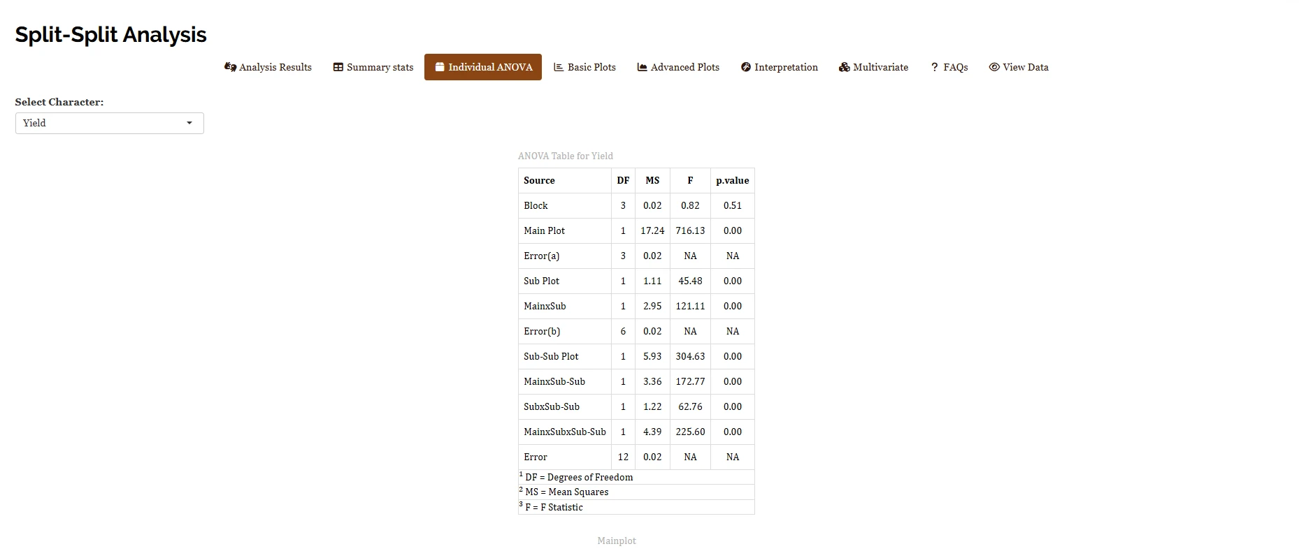
Block is non-significant for Yield here (\(F = 0.82\), \(p = 0.51\)), and that is a perfectly good outcome: it says the blocks were not so different from one another that they needed separating out. A significant Block effect is not a problem either, it means the blocking successfully removed real background variation from what would otherwise have inflated the error terms. Either way, Block is never a treatment you are trying to promote or reject; it is a check on whether local control was doing useful work.
10 Visualising the results
Tables provide the numerical results, while plots provide a visual representation of treatment differences and patterns. RAISINS groups its graphics into two sub-tabs, Basic Plots and Advanced Plots. Every plot is drawn by clicking its icon, then customised in a Plot Settings panel and exported in the format you choose.
10.1 Basic Plots
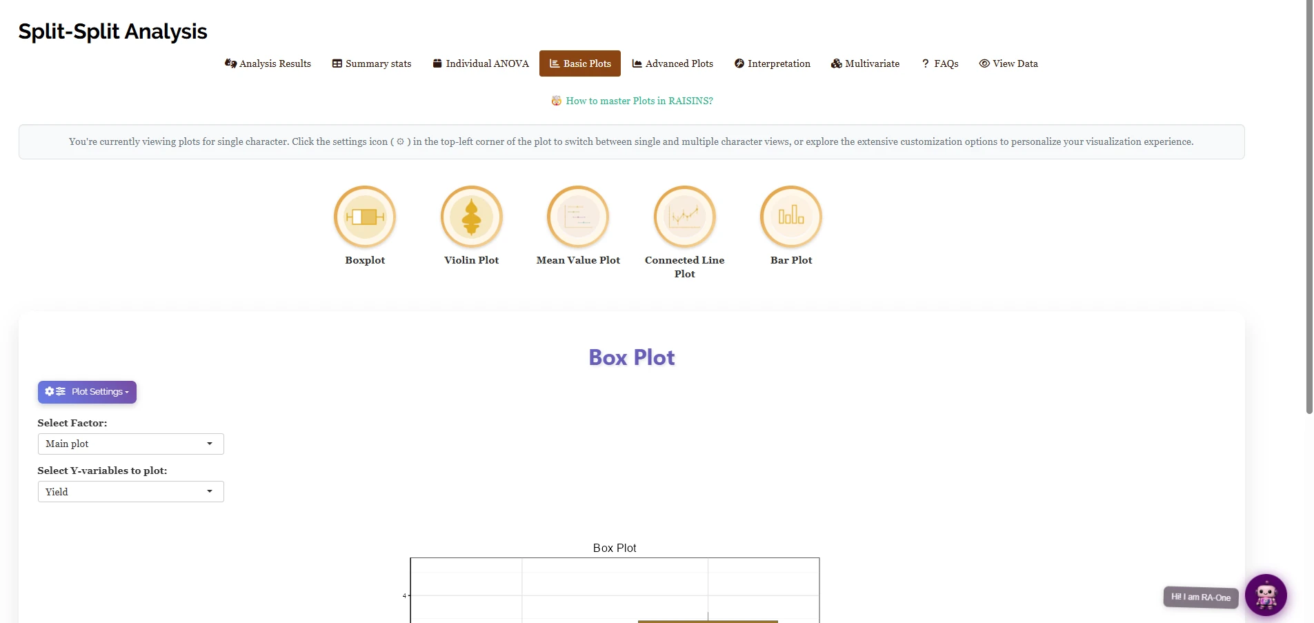
The Basic Plots tab (Figure 18) offers five everyday graphics: Boxplot, Violin Plot, Mean Value Plot, Connected Line Plot and Bar Plot. Two controls sit outside the settings panel: Select Factor, which chooses whether the x-axis shows the Main plot, the Sub plot, the Sub-sub plot, or one of their interactions, and Select Y-variables to plot, which chooses the response. A banner at the top of the tab reminds you that plots open in single-character view, and that the settings icon in the top-left corner of each plot switches between single and multiple character views. Figure 19 shows the same set of Mainplot means for Yield drawn all five ways.
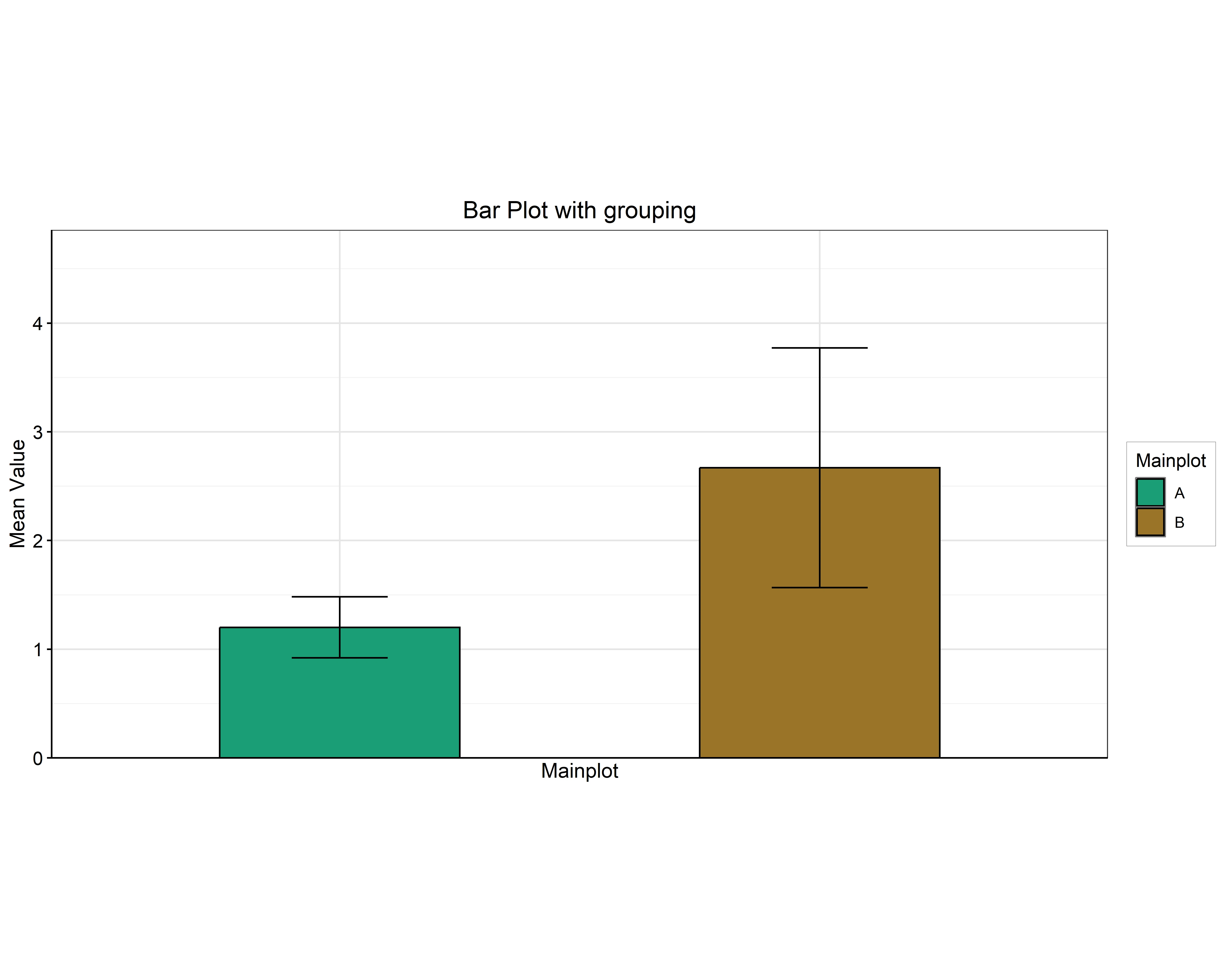
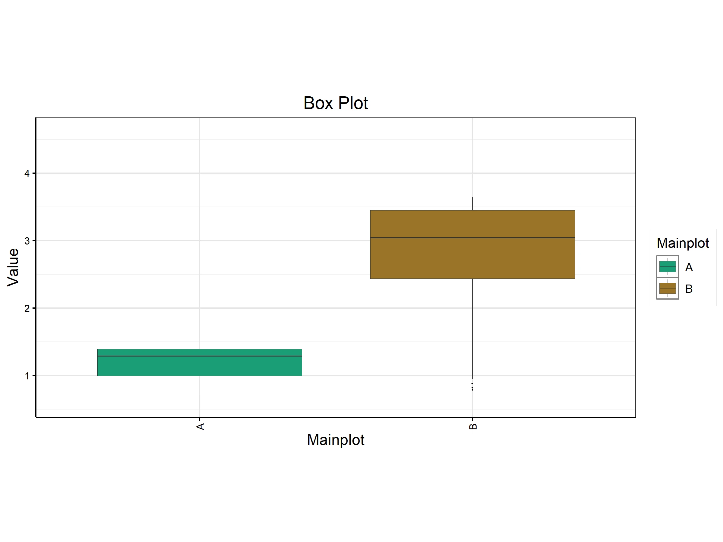
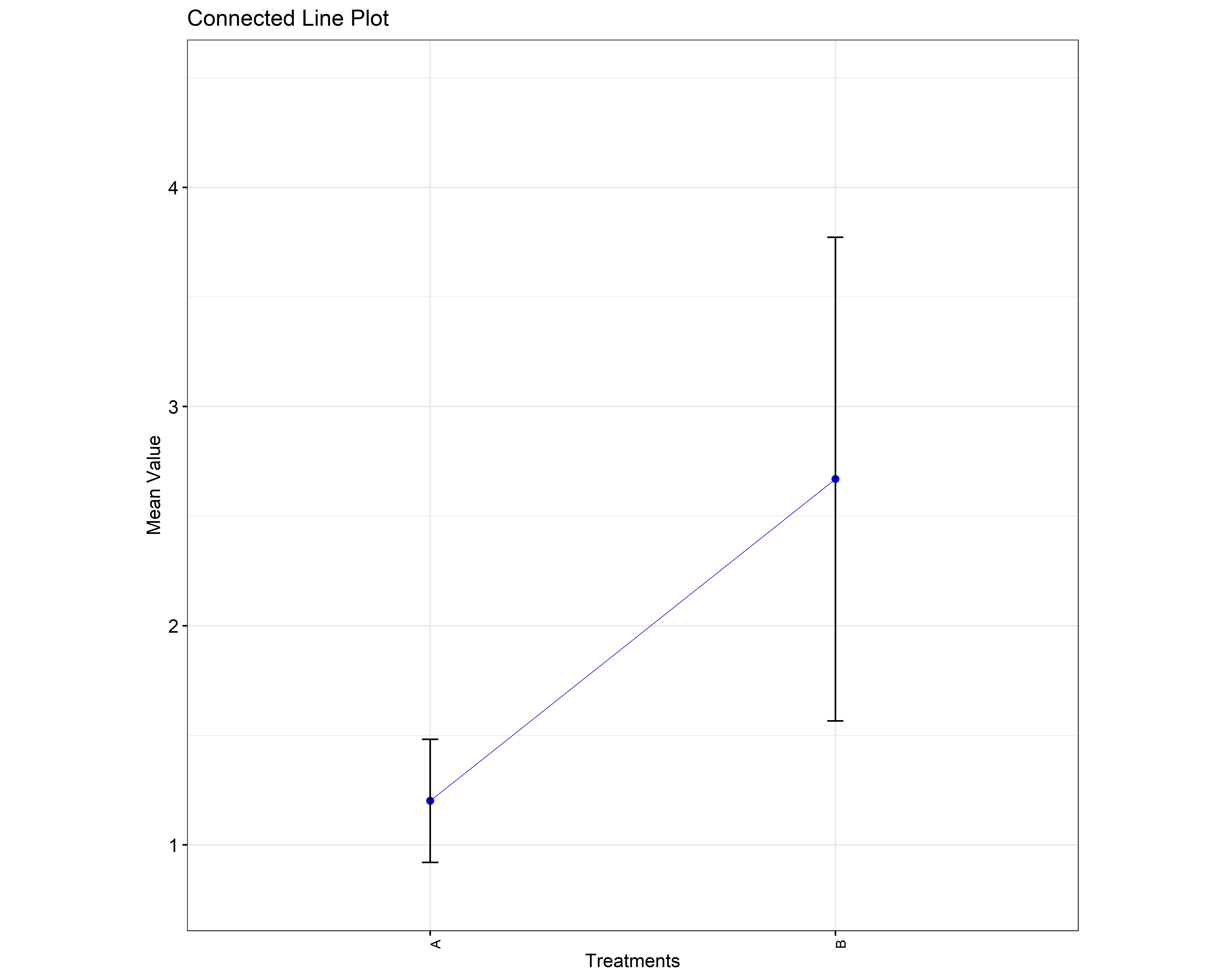
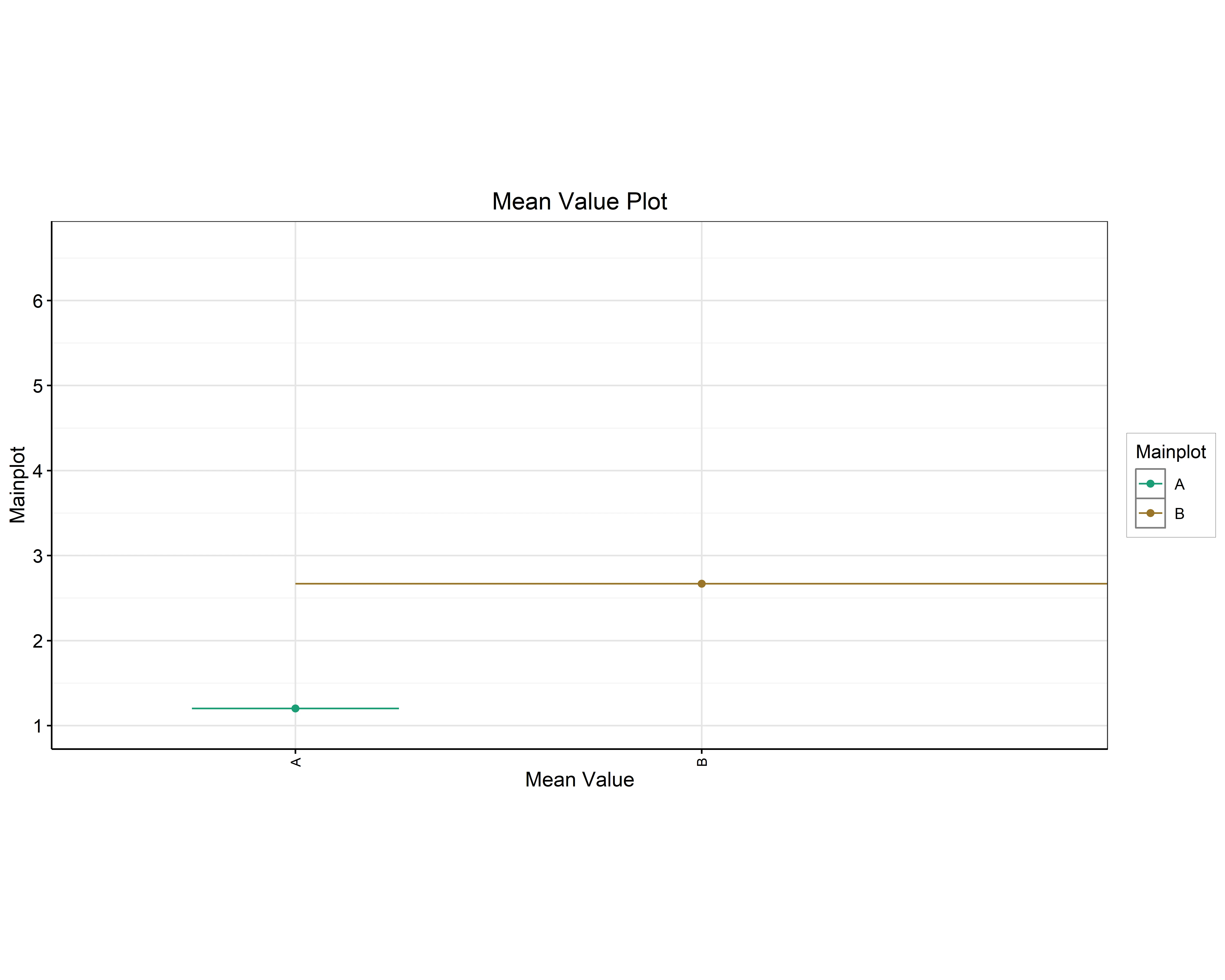
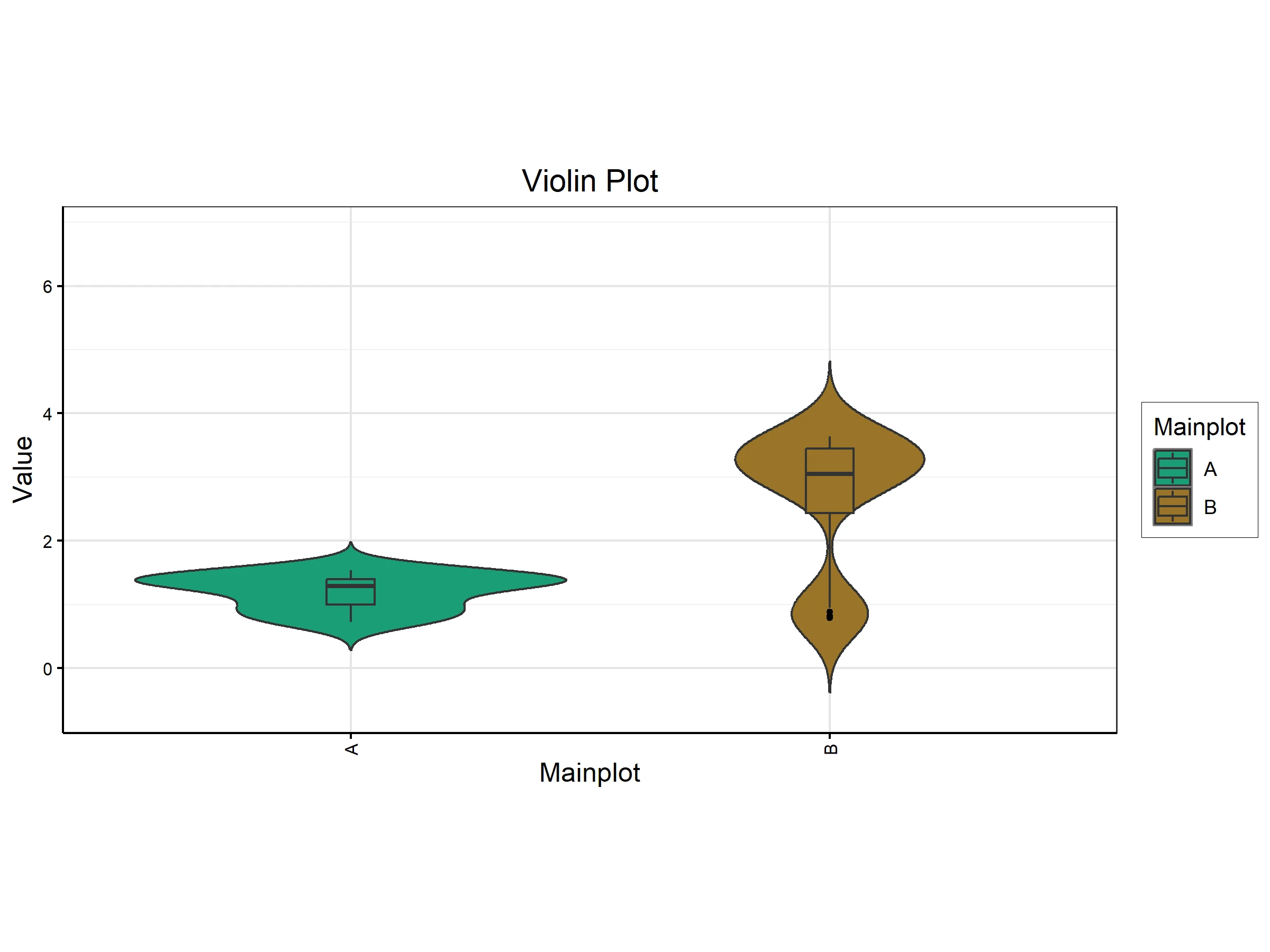
Any letters displayed above a bar, box, or point correspond to the same post-hoc groupings reported in the results tables. The plots and tables therefore represent the same statistical comparison in different forms; choose whichever format suits the purpose of your report or presentation.
10.2 Advanced Plots
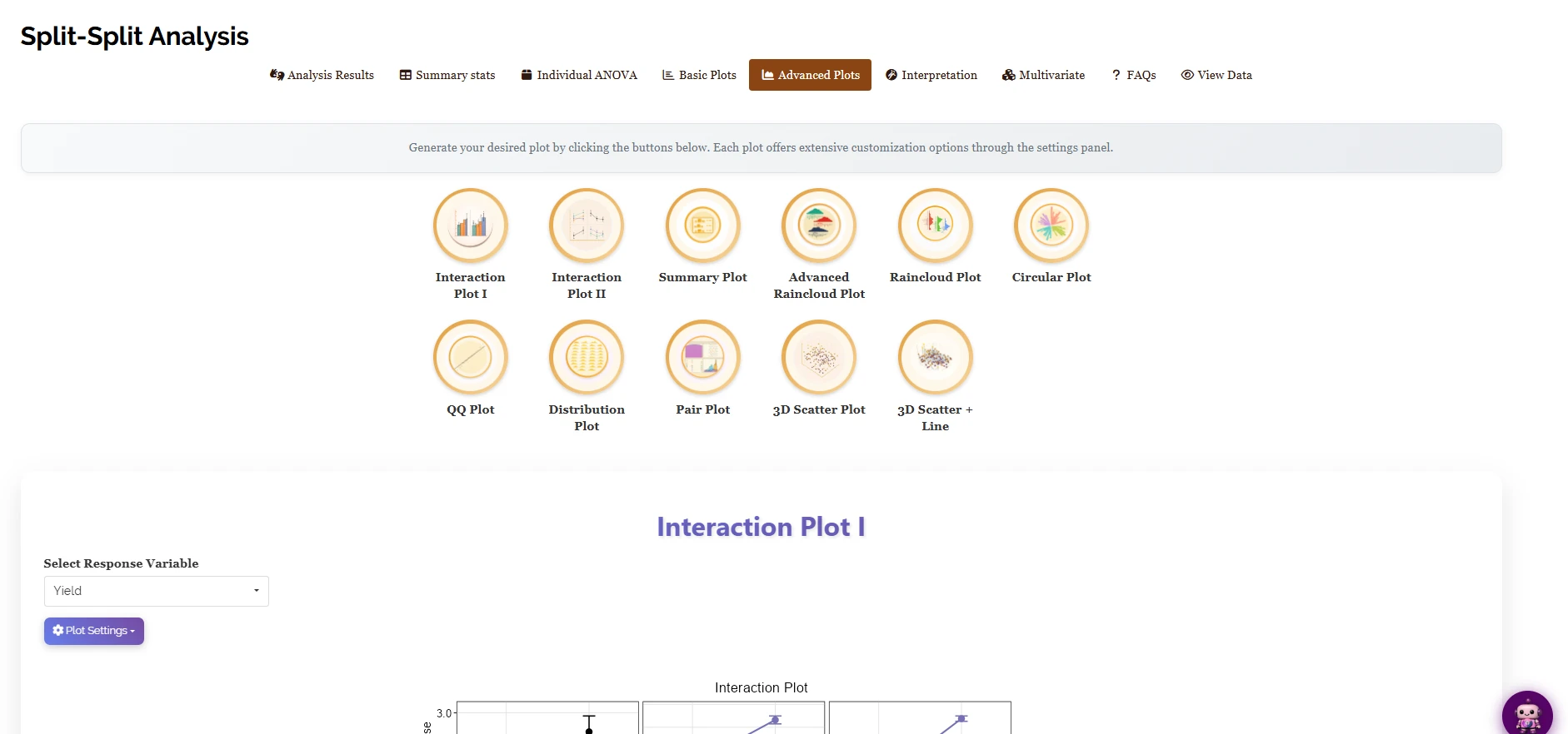
The Advanced Plots tab (Figure 20) adds specialised graphics arranged as a grid of icons: Interaction Plot I and Interaction Plot II, a Summary Plot, an Advanced Raincloud Plot and a plain Raincloud Plot, a Circular Plot, a QQ Plot, a Distribution Plot, a Pair Plot, a 3D Scatter Plot and a 3D Scatter + Line. Click any icon to draw its plot, then fine-tune it in the settings panel beneath.
The interaction plot
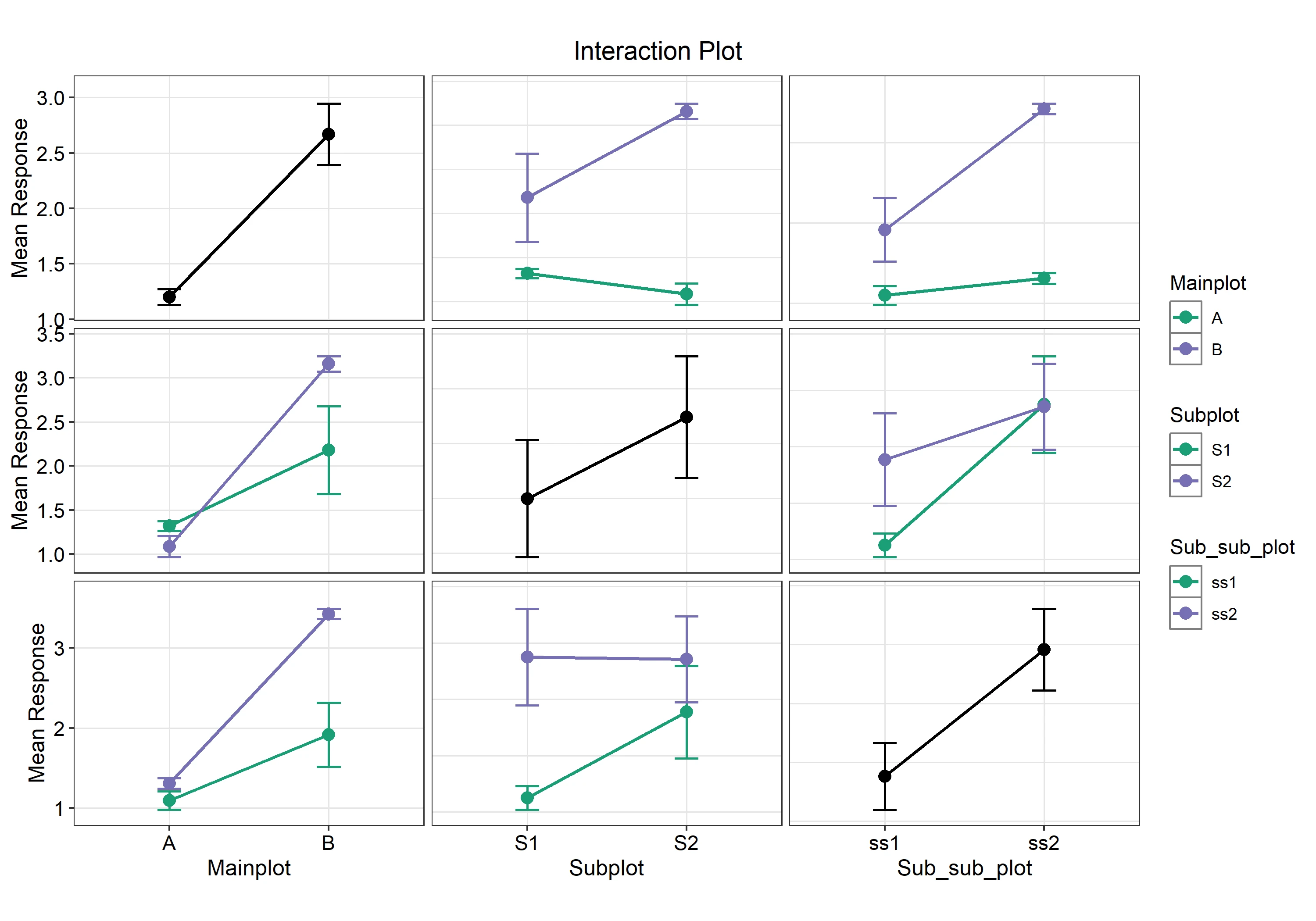
The Interaction Plot is particularly useful in a three-factor design because it lets you scan for every pairwise pattern at once. RAISINS lays it out as a \(3 \times 3\) grid: the diagonal panels (top-left, middle-centre, bottom-right) draw each factor’s own main-effect line, Mainplot, Subplot and Sub_sub_plot in turn, and the off-diagonal panels draw one factor’s mean profile across the levels of another, colour-coded by a third. Parallel lines signal no interaction between that pair; lines that cross or fan apart signal one. In Figure 21 the Mainplot panel (top-left) shows a steep rise from A to B, echoing the strong whole-plot effect already seen in Table 2, while several of the off-diagonal panels show lines that clearly diverge rather than run parallel, the visual signature of the significant two- and three-way interactions reported in Figure 12.
Rather than reading nine numbers from a results table, glance at whichever panel of Figure 21 corresponds to the two factors you care about. If its lines are close to parallel, the main-effect table is a fair summary; if they cross, go back to the interaction table (Figure 13, Figure 14, or Figure 15) for the real story, because the margins alone would be misleading.
QQ Plot and distribution checks
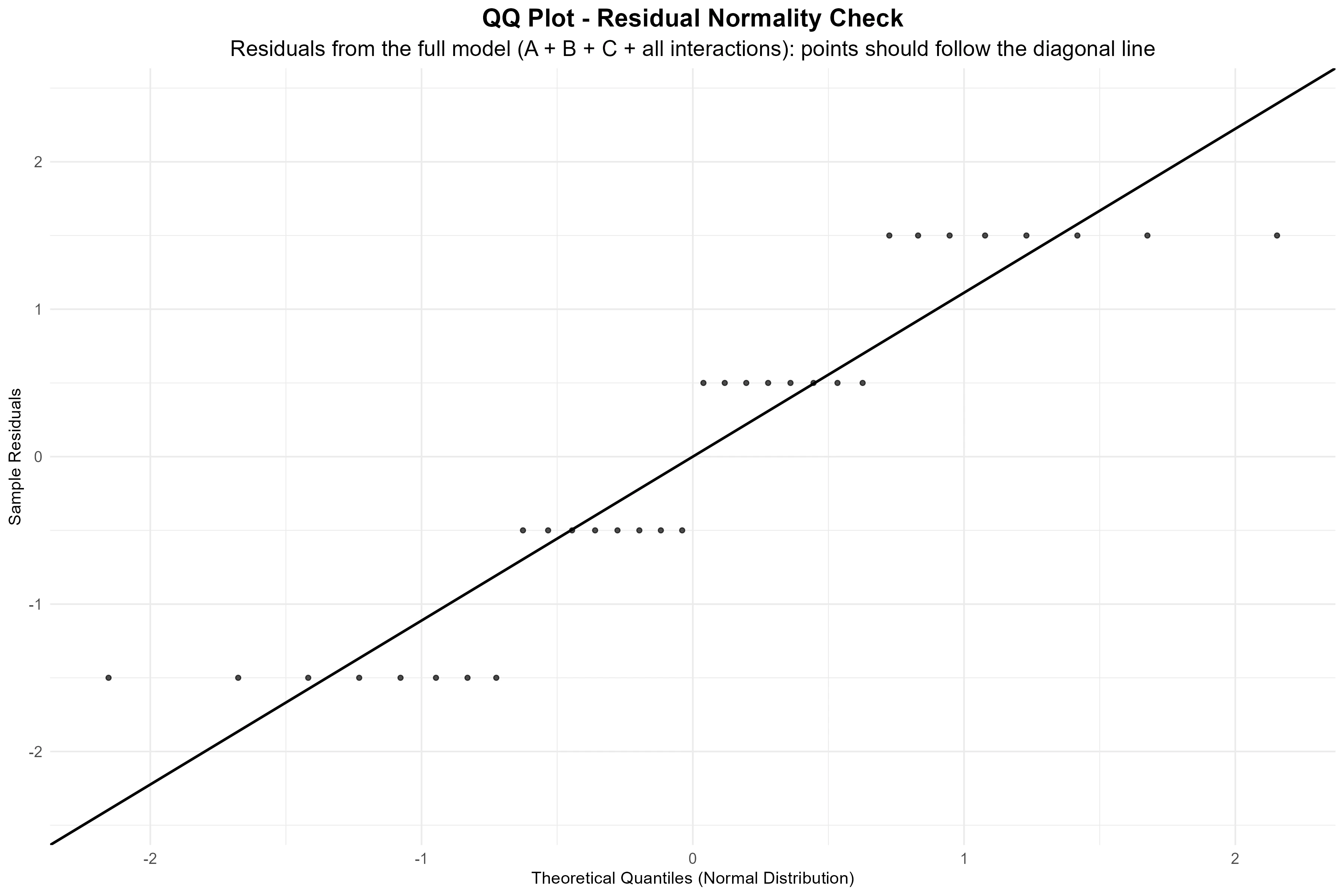
The QQ Plot checks the normality assumption behind every F-test in Figure 12, by plotting the model residuals against the quantiles of a normal distribution. Points that hug the diagonal line support normality; a pronounced curve or S-shape suggests a transformation (Section 7) may be worth considering. The Distribution Plot and Summary Plot provide complementary views of shape and of missingness/central-tendency for each response, in the same spirit as the Summary stats block in Section 9.
Raincloud, circular and 3D views
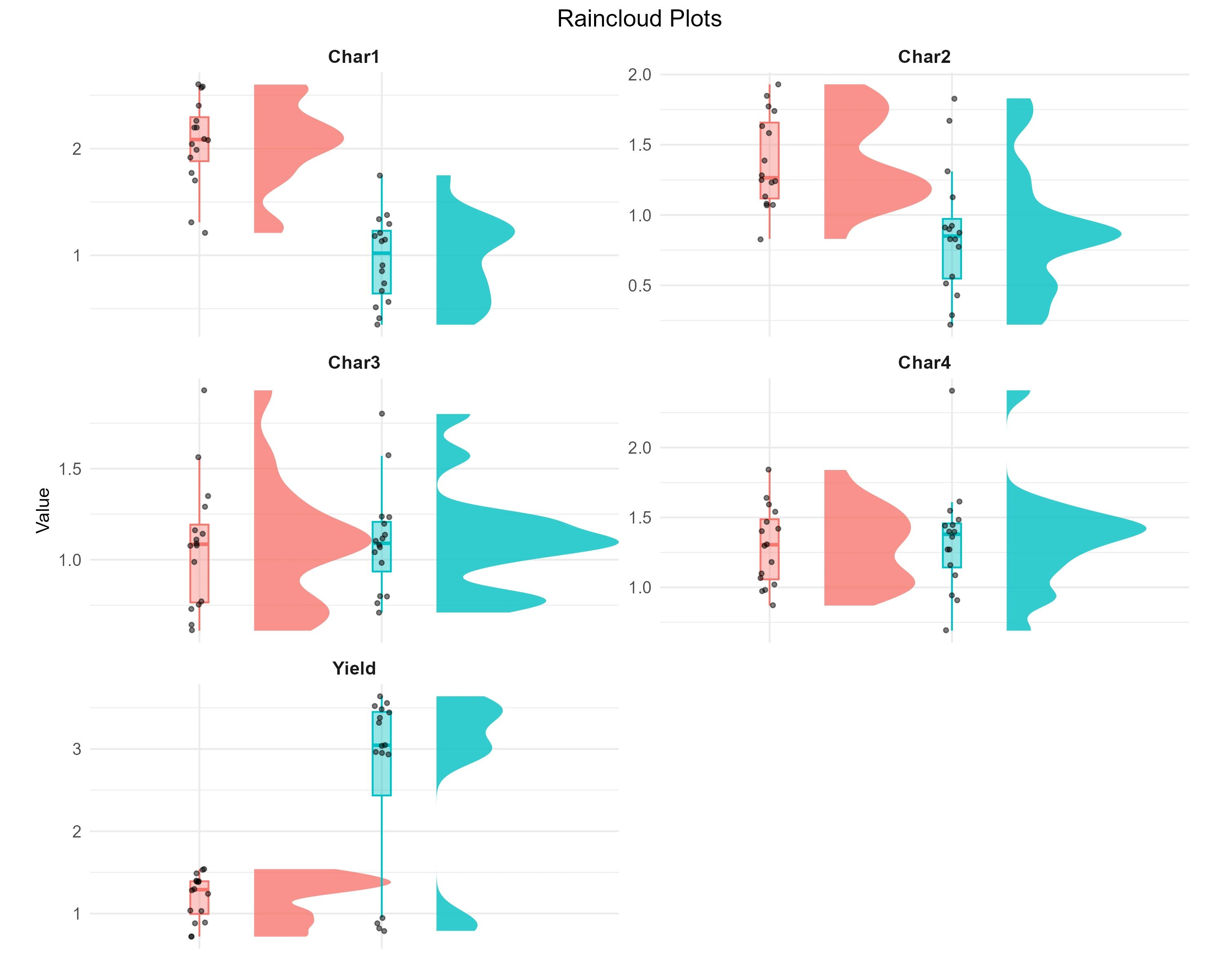
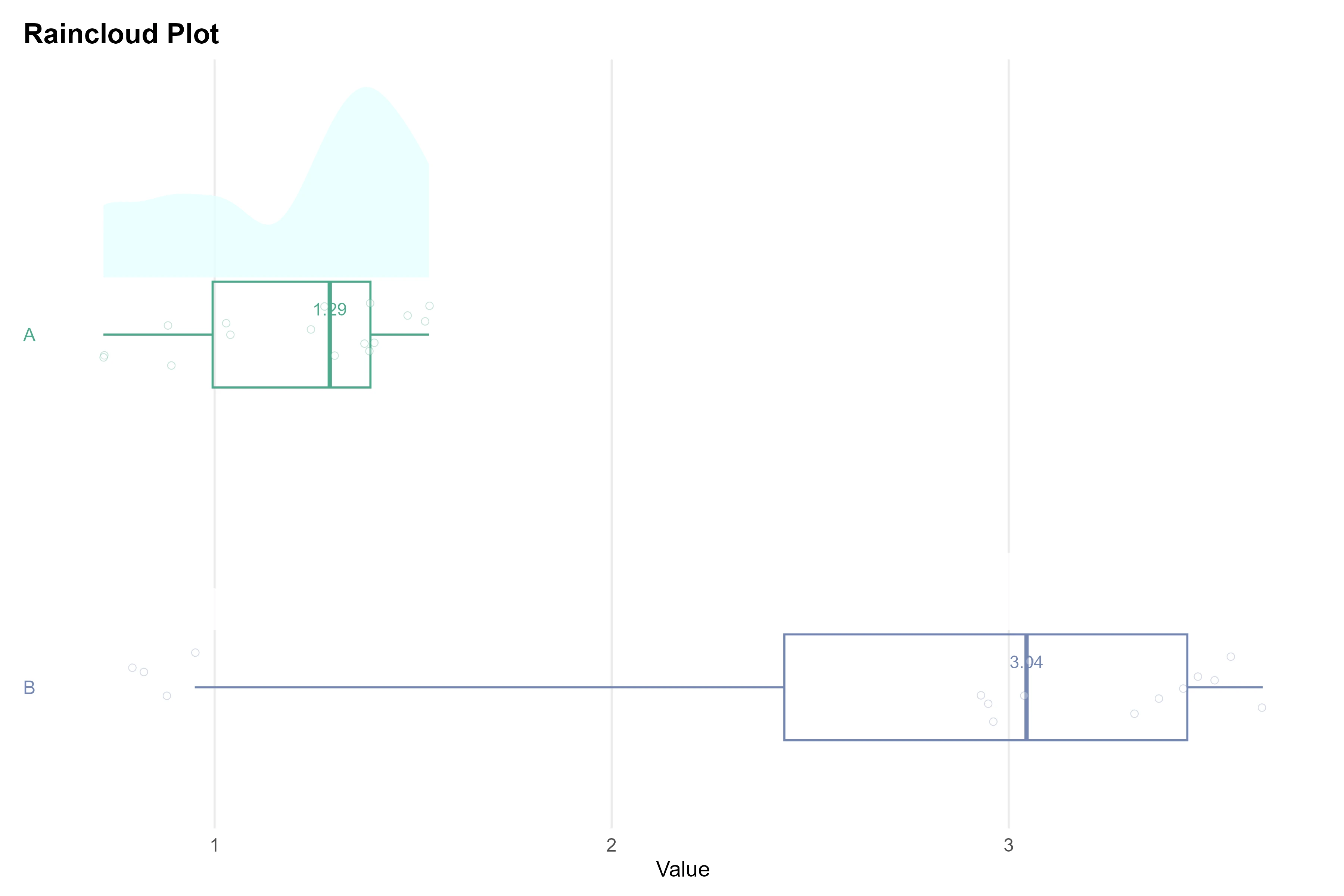
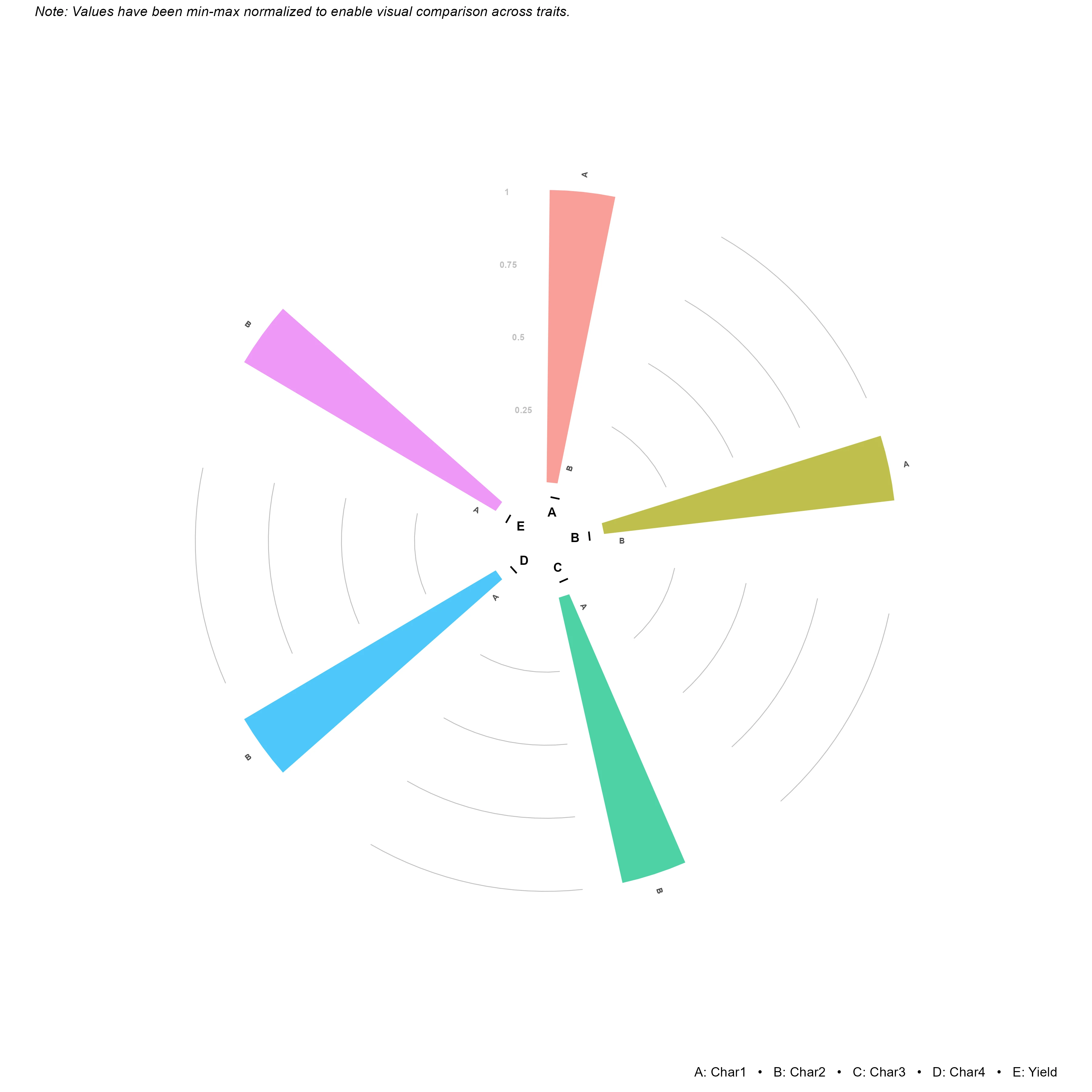
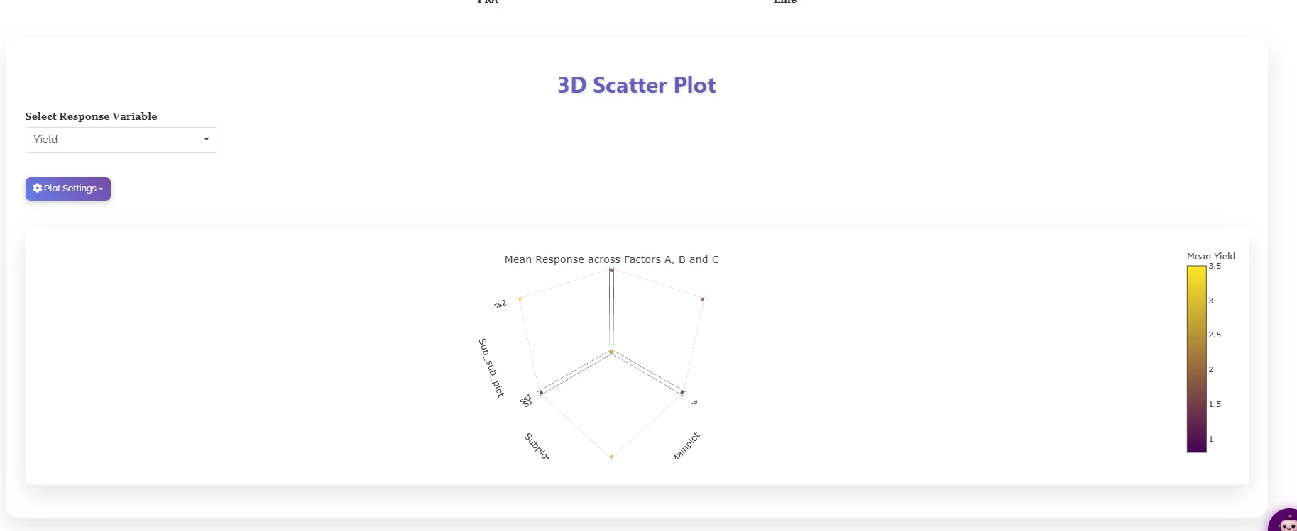
The 3D Scatter Plot and its line variant place the mean response of every whole-plot × subplot × sub-subplot combination over the three-factor space at once, which is the closest a static plot comes to showing all eight treatment combinations from Figure 15 in a single picture. The Pair Plot is the natural companion to the Multivariate tab described next, since an index is only worth building from traits that actually move together.
11 Looking at all traits together: MANOVA and the PCA index
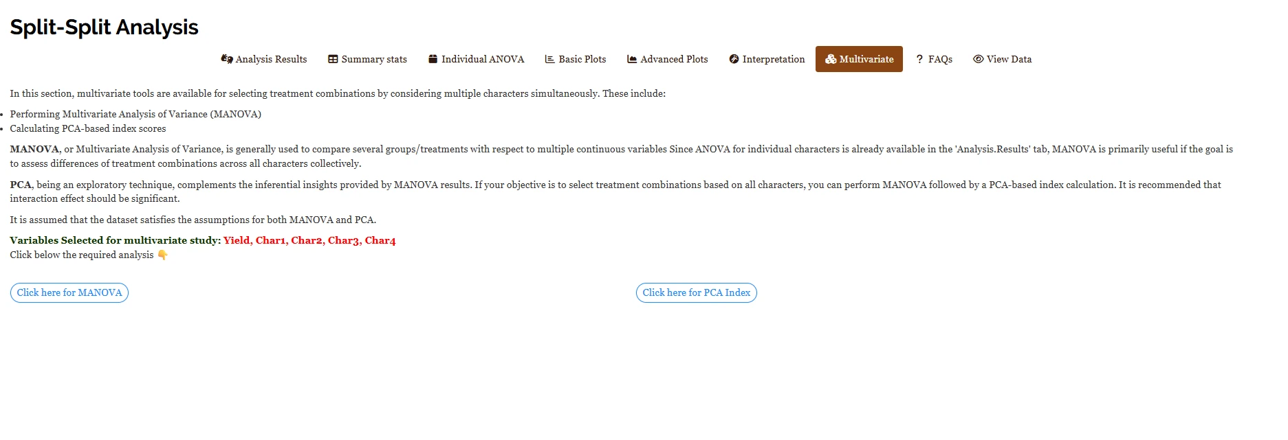
The Analysis Results tab evaluates each response separately. When several traits are measured and you want a joint test of the treatments across all of them, or a combined ranking of the eight treatment combinations, the Multivariate tab provides two tools, MANOVA and a PCA-based index score (Figure 25). MANOVA is generally used to test whether groups differ on several continuous variables considered together; since ANOVA for each individual character is already available under Analysis Results, MANOVA is primarily useful for assessing differences between treatment combinations across all characters collectively. PCA, an exploratory technique, complements the inferential MANOVA result: if the goal is to select treatment combinations based on all characters at once, RAISINS recommends running MANOVA first and following it with a PCA-based index, ideally when the interaction effect is significant.
11.1 MANOVA across all responses
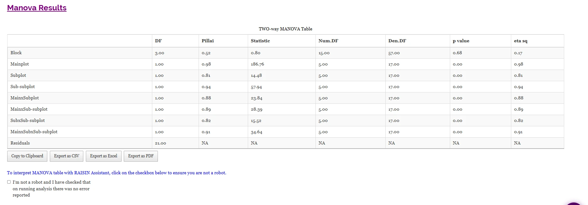
Every treatment source in Figure 26 is significant at \(p = 0.00\) when all five traits are considered jointly: Mainplot (Pillai \(= 0.98\), \(F = 186.76\), \(\eta^2 = 0.98\)), Subplot (Pillai \(= 0.81\), \(F = 14.48\), \(\eta^2 = 0.81\)), Sub-subplot (Pillai \(= 0.94\), \(F = 57.94\), \(\eta^2 = 0.94\)), and all four interactions, MainxSubplot (\(\eta^2 = 0.88\)), MainxSub-subplot (\(\eta^2 = 0.89\)), SubxSub-subplot (\(\eta^2 = 0.82\)) and MainxSubxSub-subplot (\(\eta^2 = 0.91\)). Block, by contrast, is non-significant (Pillai \(= 0.52\), \(F = 0.80\), \(p = 0.68\)), matching the univariate result already seen for Yield in Section 9. The very high partial eta-squared values here, several above 0.90, reflect that Yield alone already showed enormous separation between treatments (Table 2), and MANOVA is picking that up across the whole trait set at once.
MANOVA’s significant result for every treatment source does not mean every individual trait is significant for every source, Char4 was non-significant throughout Figure 12. MANOVA asks whether the treatment combinations differ on the combination of traits considered jointly; a trait-by-trait breakdown still needs the univariate tables in Section 8.
11.2 PCA-based index score
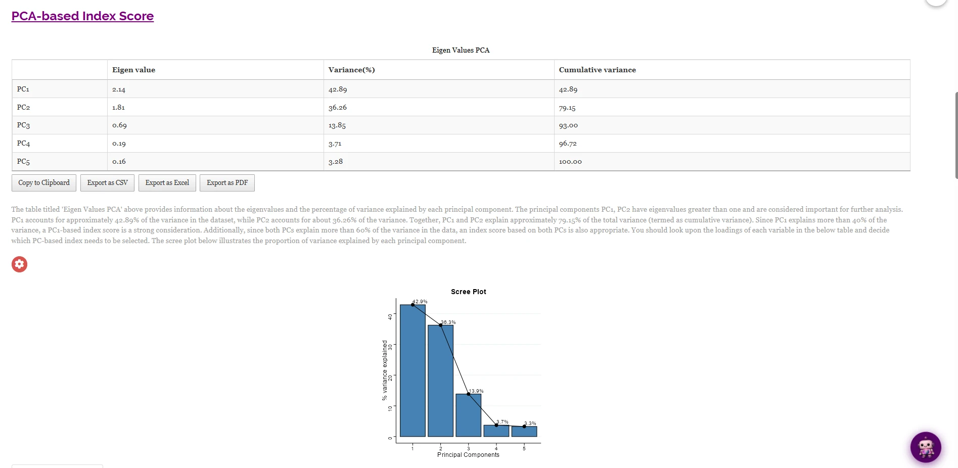
The eigenvalue table (Figure 27) helps decide how many principal components to retain. Here PC1 has an eigenvalue of 2.14 and accounts for 42.89% of the variance, and PC2 has 1.81 for a further 36.26%; together the first two components explain 79.15%. Both exceed the conventional eigenvalue-of-one threshold, and RAISINS notes that because both exceed 60% cumulatively, an index built on either, or both, is meaningful. PC3 (0.69, 13.85%) falls below the threshold, and by PC5 the cumulative variance has reached 100%. The accompanying scree plot shows a fairly gentle decline from PC1 to PC2, meaning the variation in this five-trait dataset is not dominated by a single component.
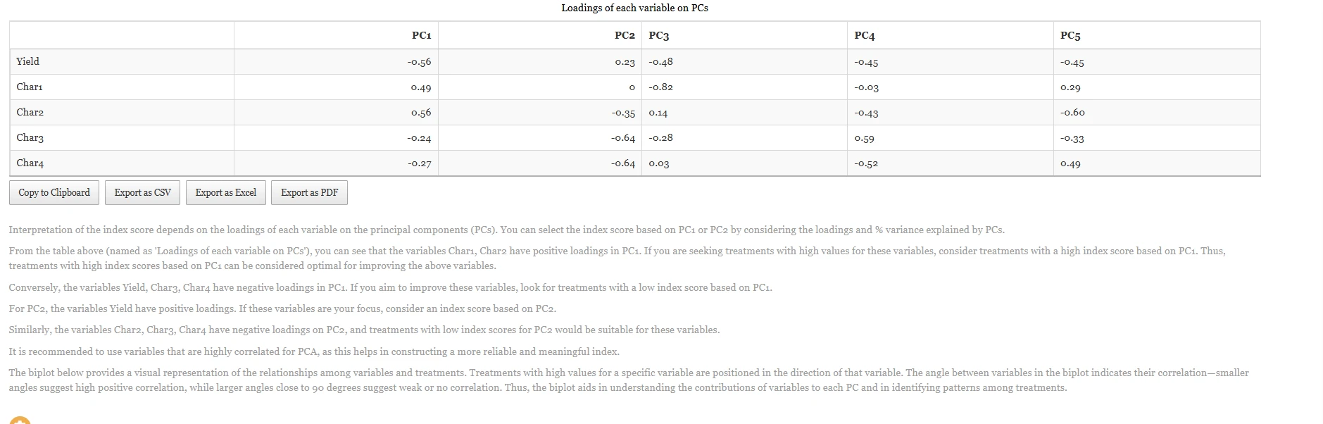
The loadings table (Figure 28) tells you what each component means, and should be read before any index is used. On PC1, Char1 (0.49) and Char2 (0.56) load positively while Yield (−0.56), Char3 (−0.24) and Char4 (−0.27) load negatively, so a treatment with a high PC1 score tends to be strong on Char1 and Char2 but weak on Yield, Char3 and Char4. On PC2, only Yield loads positively (0.23); Char2, Char3 and Char4 all load negatively, most strongly Char3 and Char4 (both −0.64). There is no universally “good” end of a component, only an end that matches the traits you are trying to improve.
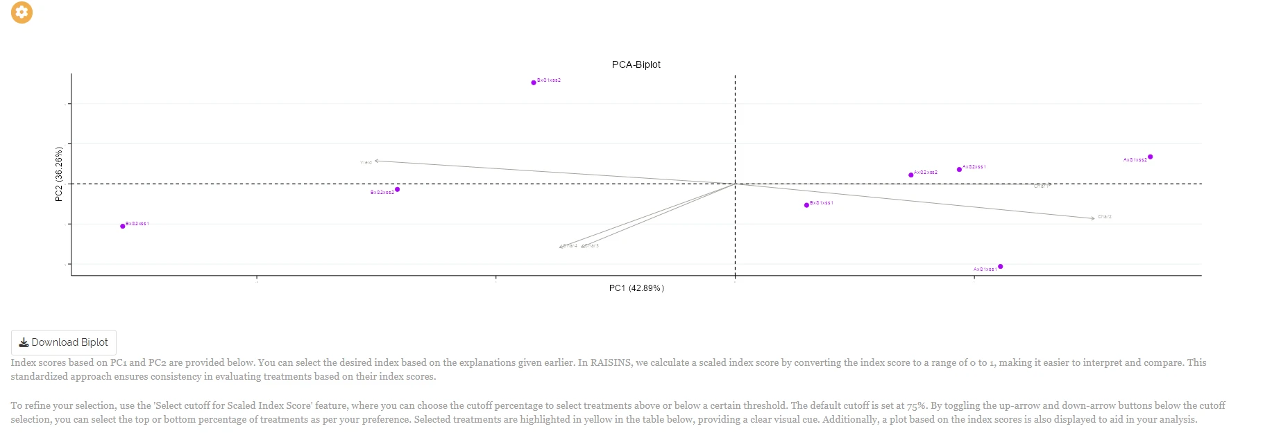
RAISINS then converts the selected principal component into a scaled Index Score for each of the eight treatment combinations shown in Figure 29, AxS1xss1, AxS1xss2, AxS2xss1, AxS2xss2, BxS1xss1, BxS1xss2, BxS2xss1 and BxS2xss2, scaling the values to a 0–1 range so combinations can be compared directly. The Select cutoff for Scaled Index Score control decides how many of the eight are highlighted as selected, and the cutoff can be moved with the up/down arrows to select the top or bottom percentage of treatments as needed.
The PCA index is exploratory, not inferential. It produces an ordering of treatment combinations, but no p-value and no critical difference. Nothing in Figure 29 contradicts the MANOVA and ANOVA findings above, the index answers a different question, “which combinations look best across all traits at once”, rather than “which combinations differ significantly.” Use it to shortlist candidates for a follow-up experiment, always alongside, never instead of, the significance tests in Section 8.
The biplot and the score table each name the principal component they are based on, and can be switched independently. Since PC1 and PC2 weight the five traits in genuinely different directions, as Figure 28 shows, always confirm which component produced the ranking you are about to quote.
12 Interpretation
RAISINS also provides a plain-language interpretation of the statistical results. Open the Interpretation sub-tab, tick the confirmation box, “I’m not a robot and I have checked that on running analysis there was no error reported”, and click Click here for interpretation to generate a summary (Figure 30).
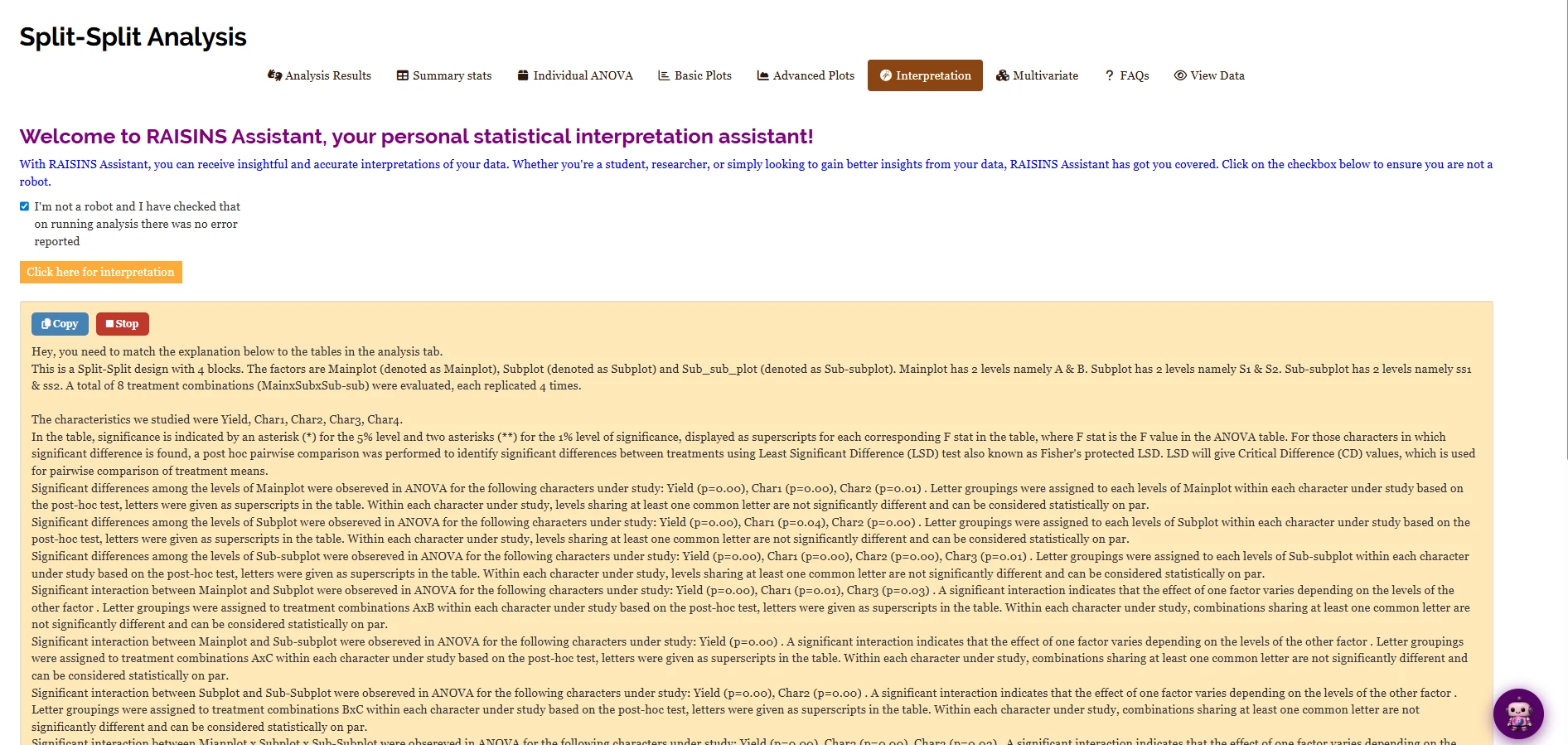
RAISINS restates the design, “This is a Split-Split design with 4 blocks. The factors are Mainplot (denoted as Mainplot), Subplot (denoted as Subplot) and Sub_sub_plot (denoted as Sub-subplot). Mainplot has 2 levels namely A & B. Subplot has 2 levels namely S1 & S2. Sub-subplot has 2 levels namely ss1 & ss2. A total of 8 treatment combinations (MainxSubxSub-sub) were evaluated, each replicated 4 times,” names the post-hoc test, and then reads each character and each source in turn: which whole-plot, subplot and sub-subplot effects were significant, which of the four interactions were significant, and for which characters the letter groupings apply. The generated text for this dataset reports significant Mainplot, Subplot and Sub-subplot effects for Yield, Char1 and Char2, a significant A × B interaction for Yield, Char1 and Char3, and a significant A × C interaction for Yield, all matching Figure 12 exactly, before continuing on to the B × C and three-way rows. The text is written to be pasted almost directly into a results section.
The interpretation is generated from the same computation as the tables, so use it as a guide, not a substitute. Read it with Figure 12 and Figure 15 open beside it, the numbers in the prose should match the numbers in the tables exactly, which is your quickest check that the whole-plot, subplot and sub-subplot columns were selected the right way round on the Analysis tab.
13 Chat with your data using RA-One
RA-One is the built-in conversational assistant for the split-split-plot module, available from the RA-One tab. It answers questions using the results generated from your own analysis rather than generic statistical explanations, so every number it quotes comes from what the module has calculated, and it tells you when a value is not available rather than guessing. All of its answers are in plain English, without code or software commands.
Once your results are loaded, RA-One offers quick-start prompts such as Guide me through my results, Interpret results, Best treatment, and Report results, and you can also type your own question, for example “Is the three-way interaction significant for Char2?” or “Which sub-subplot treatment gives the highest Yield under whole plot B?”. A status line in the corner confirms that the analysis context has been loaded.
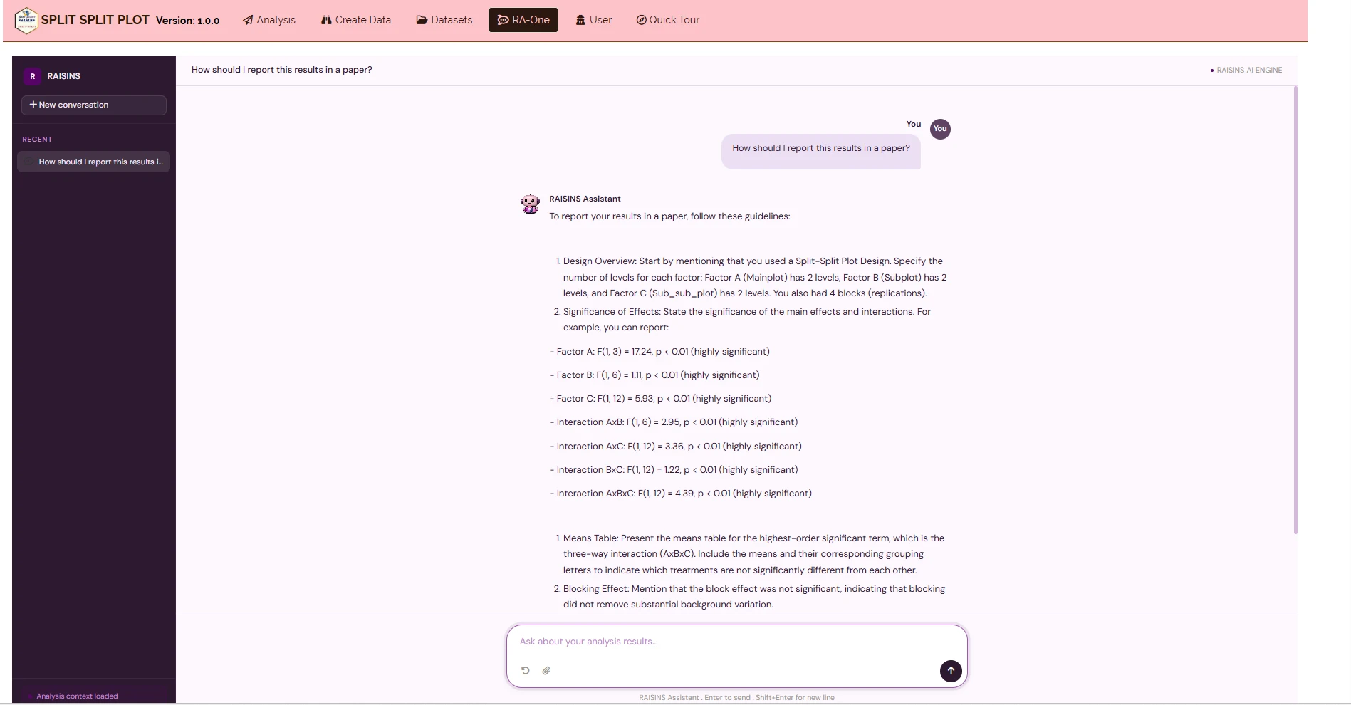
The Report results prompt is especially useful for a split-split-plot, because the reporting conventions involve three factors and their interactions rather than one. Asked “How should I report this results in a paper?”, RA-One returns an ordered checklist (Figure 31): state that the design was a Split-Split Plot Design with Factor A (Mainplot) at 2 levels, Factor B (Subplot) at 2 levels and Factor C (Sub_sub_plot) at 2 levels, with 4 blocks; report the significance of every main effect and every interaction with its F and p value, for example “Factor A: F(1, 3) = 17.24, p < 0.01” through “Interaction AxBxC: F(1, 12) = 4.39, p < 0.01”; present the means table for the highest-order significant term, here the three-way A × B × C interaction, together with its letter grouping; and mention the blocking effect explicitly, here noting that it was not significant, so blocking did not remove substantial background variation.
The same chat interface can also prepare data. It can generate a correctly formatted design template (Section 6.4), including a check of the error degrees of freedom for all three strata, or provide a model dataset (Section 6.3) for practice and demonstration.
Within a single conversation, RA-One can interpret your results, build a data template with its error-df check, fetch a model dataset, and help you draft the write-up, including which of the seven interaction terms belongs in your final table. Most of a routine split-split-plot session can be conducted without ever leaving the chat window.
14 FAQs
The module includes a dedicated FAQs sub-tab with explanations of common questions and guidance on the available features. Three questions are particularly important for a first analysis because they are specific to a three-stratum design: which factor should go on the main plot, which on the sub plot, and which on the sub-sub plot?, which restates the practical rule from Section 1; why are there so many CD values?, which covers the same ground as Section 8.1 from the reporting side; and which interaction table should I report when several are significant?, which restates the “report the highest-order significant term” rule seen in Figure 31. The same explanations are always one click away inside the analysis itself, through the Know more button beside each CD selector.
15 View data
View Data is the primary diagnostic tool for ensuring data integrity before analysis (Figure 32). When you upload your dataset, RAISINS runs an automated Health Check: the treatment columns, Mainplot, Subplot and Sub_sub_plot, are highlighted yellow and the response columns are highlighted green. If both conditions hold, spaces between numbers or incorrect decimal points would otherwise show up as yellow highlighting in a numeric column, the file is in good health. The instructions panel at the top of the tab spells out exactly what to look for and how to correct it.
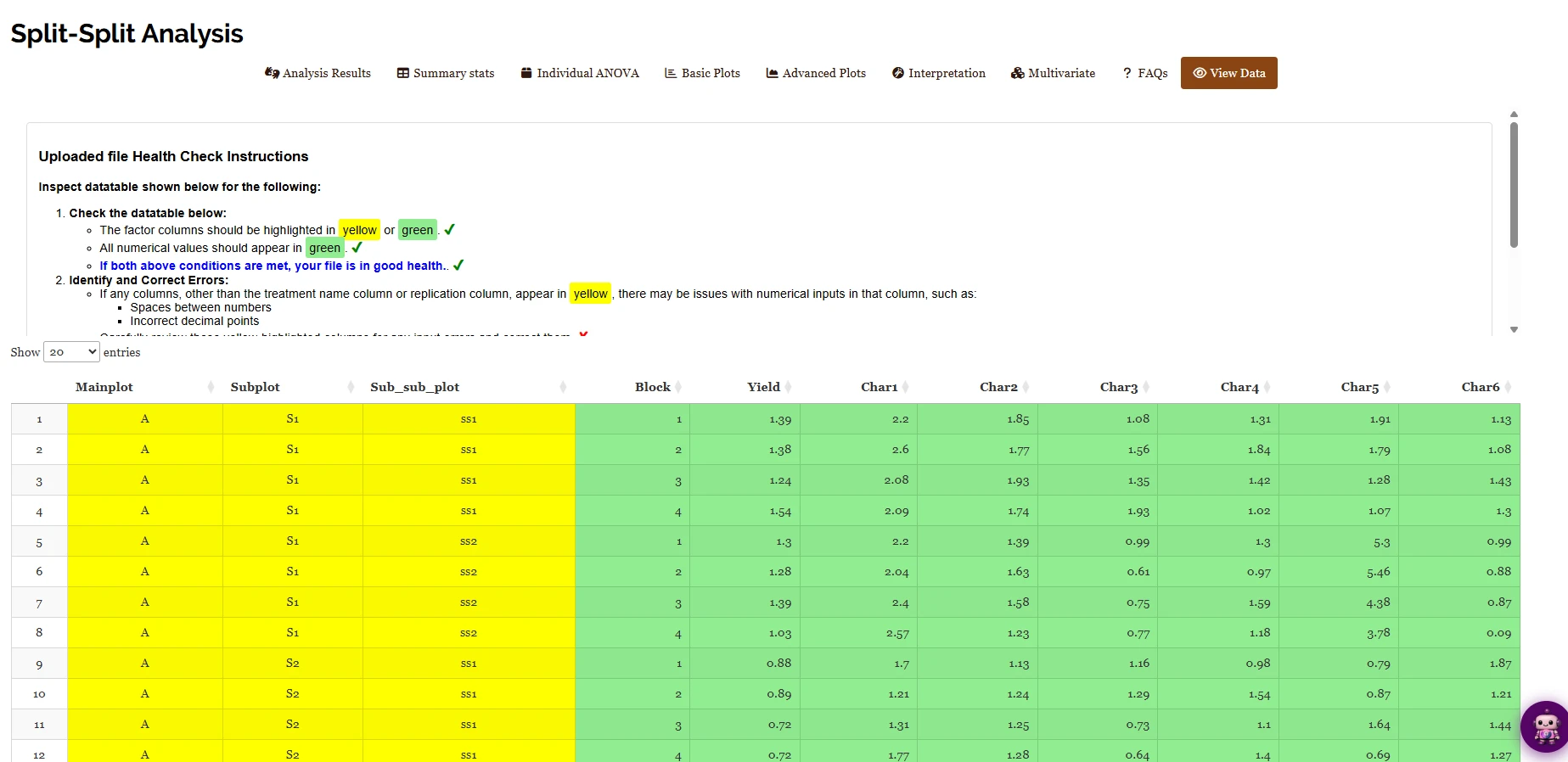
For a split-split-plot it also checks the property that defines the design: that every sub-subplot treatment appears once inside every whole-plot × subplot × block combination, and that every subplot treatment appears once inside every whole-plot × block combination. If a sub-subplot is missing from one subplot, a subplot is missing from one whole plot, or a treatment label is spelled two different ways, the nesting breaks at that level, the corresponding error term can no longer be cleanly separated, and the critical differences of Section 8.1 stop being exact. Fix anything flagged here before trusting the results, and cross-check the Missing figures against the Summary stats block in Section 9.
16 Wrapping up
A split-split-plot design is appropriate when three factors differ in how difficult they are to randomise, so much so that a single split-plot is not enough to accommodate them. The resulting three-stage randomisation creates three types of experimental unit and, consequently, three error terms, Error(a), Error(b) and Error(c). These error terms lead to a whole family of critical differences: CD(A), CD(B) and CD(C) for the single-factor comparisons, CD[A(B)] and CD[B(A)] for whole-plot-versus-subplot comparisons, CD[B(C)] and CD[C(B)] for subplot-versus-sub-subplot comparisons, and CD[AB(C)], CD[BC(A)] and CD[CA(B)] for the three-way table. When interpreting the results, identify the error term used for each F-test, and select the critical difference whose definition, quoted in full in Section 8.1, matches the comparison you actually want to make.
Let’s break this down with the working example. Yield showed every source significant, so the report for Yield leans on the eight-cell three-way table (Figure 15): BxS1xss2 and BxS2xss2 are the top performers, sharing letter a under CD[BC(A)], the most conservative yardstick available, because that letter grouping already survives a comparison that crosses whole plots. Char1, by contrast, showed no interaction involving C, so its story is told correctly by the whole-plot, subplot and sub-subplot margins together with the A × B table, not by the eight-cell breakdown. Reporting the wrong level of detail, margins for Char2 and Char3, or the three-way table for Char1, would misrepresent what the data actually show.
The design also carries an important limitation: the whole-plot factor is tested using the fewest degrees of freedom (3 in the working example) and therefore generally has the lowest precision of the three factors, while the sub-subplot factor, tested on the most degrees of freedom (12), has the highest. A split-split-plot design is most appropriate when this loss of precision on the hardest-to-change factor is an acceptable price for the practical convenience it buys. If only two factors differ in how hard they are to change, the split-plot module is the right tool. If all factors can be randomised freely to small experimental units, the three-factor factorial CRD module may be more appropriate, and when natural blocks are present without any nested randomisation constraint, the three-factor factorial RBD module applies instead. RA-One and the support resources are available when further guidance is required.
