Endogenous Switching Regression
1 The Concept
Understanding adoption, selection bias, and treatment effects

1.1 Does the improved seed make a difference?
Does using an improved seed variety increase a farmer’s yield?
Who adopts?
Some farmers try the improved seed. Others continue with their usual variety.
What do we observe?
We see the seed each farmer chose and the yield they harvested.
Why is comparison difficult?
The farmers choosing the new seed may also have more experience, better irrigation, or larger farms.
What do we need?
A method that accounts for why farmers choose, so we can isolate the seed’s true effect.

1.2 Why comparing average yield can be misleading
Imagine that the more experienced farmers are also the first to try the improved seed.
They may get higher yields because of:
- the improved seed, and
- their greater experience.
How much of their higher yield comes from the seed, and how much comes from their experience?
This mixing of influences is selection bias. It can make the seed’s benefit look larger or smaller than it really is.

1.3 What we measure and what we miss
What the dataset tells us: education, farm size, and irrigation access. These measured characteristics can enter the model as covariates.
What the dataset may miss: farming skill, motivation, or willingness to take risks.
For example, a motivated farmer may be more willing to try new seed and more attentive to crop management.
ESR models the connection when hidden factors influence both adoption and yield.

1.4 The missing comparison: the counterfactual
Imagine a farmer who used the improved seed this season. We know the yield they harvested.
What would that same farmer, in that same season, have harvested without adopting?
That missing outcome is the counterfactual.
A neighbour’s yield cannot simply fill the gap: their land, experience, and resources may differ.
ESR uses the data and its assumptions to estimate this missing comparison.

1.5 What “endogenous switching regression” means
Endogenous: hidden influences on the choice may also affect the outcome. For example, motivation may influence both adoption and yield.
Switching: the choice places a farmer in one of two groups, called regimes: adoption or non-adoption.
Regression: the model describes how yield varies with characteristics such as irrigation and farm size within each group.
ESR brings the choice and the two outcome relationships into one connected model.
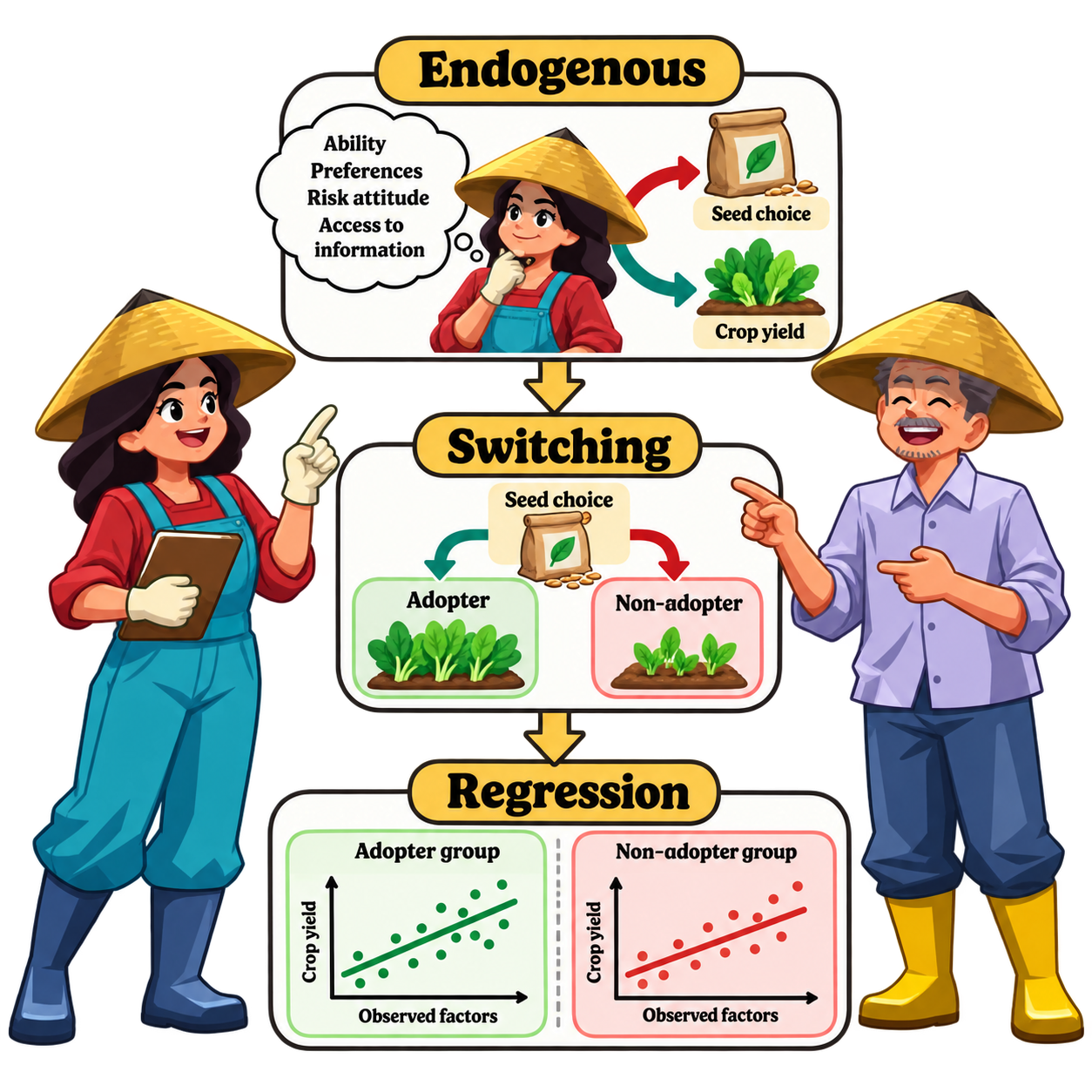
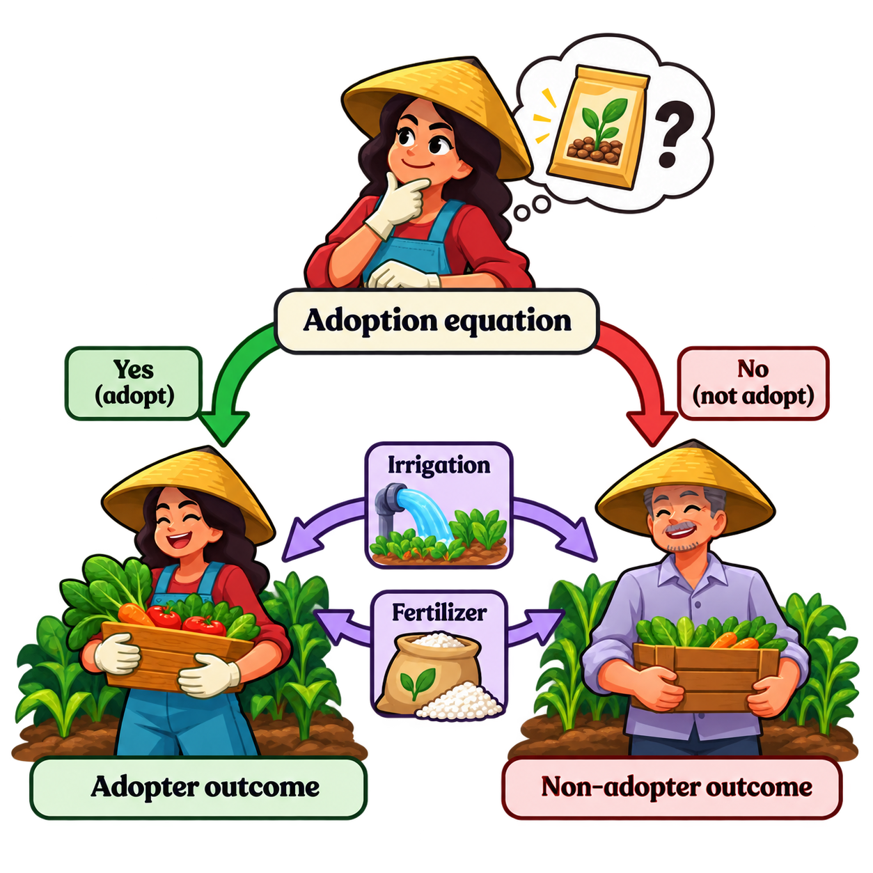
1.6 Why ESR uses three equations
One adoption equation explains who is more likely to adopt. It uses a probit model, which is suitable for a yes-or-no decision.
One outcome equation for adopters describes how their yield relates to factors such as irrigation and fertilizer use.
One outcome equation for non-adopters describes those relationships among farmers using the usual variety.
The relationships can differ. For example, irrigation may be associated with a larger yield increase under one variety than the other.
Methodological foundation: Lokshin and Sajaia (2004).
1.7 Why an instrument helps
An instrument helps explain why a farmer adopts. To be useful for identifying the adoption effect, it must also meet two conditions:
- It has no separate effect on yield apart from its influence through adoption.
- It does not reflect hidden influences on yield, after accounting for the controls.
For example, distance to a seed dealer needs careful justification. It may influence adoption, but it may also affect access to fertilizer or markets.
A useful predictor of adoption is not necessarily a valid instrument.
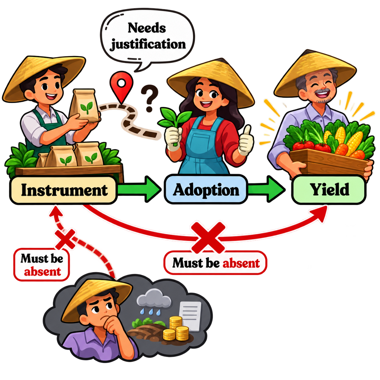
A credible excluded instrument strengthens identification. The standard normal ESR model can also rely on functional-form nonlinearity without an exclusion, but this increases dependence on parametric assumptions. Exclusion and instrument exogeneity require substantive reasoning.
1.8 How the selection correction works
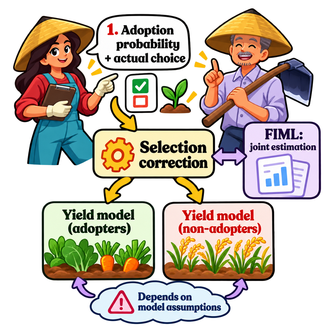
The adoption model first estimates how likely each farmer is to choose the improved seed.
In two-step ESR, that probability and the farmer’s actual choice provide a selection correction term, called the inverse Mills ratio.
This term helps the yield models account for the fact that farmers selected themselves into the two groups.
Full-information maximum likelihood (FIML) takes a joint approach: it fits the adoption and yield relationships together.
The correction works only as well as the model’s assumptions describe the data.
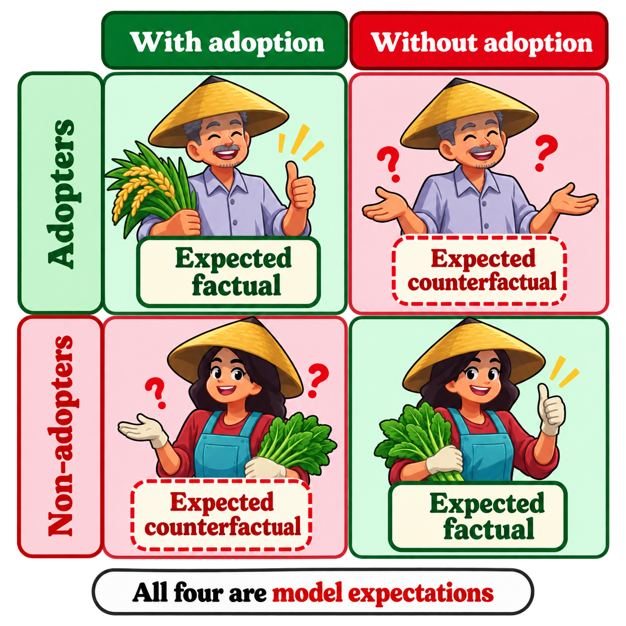
1.9 The four expected outcomes
For farmers who adopted, ESR considers:
- Their expected yield with adoption.
- Their expected yield without adoption: the counterfactual.
For farmers who did not adopt, ESR considers:
- Their expected yield without adoption.
- Their expected yield with adoption: the counterfactual.
Each is an expected yield from the model. A prediction describes what the model expects, rather than reproducing each farmer’s harvest exactly.
1.10 ATT: the effect for adopters
ATT means Average Treatment effect on the Treated. Here, “treated” means farmers who adopted.
The comparison stays with the same adopter group: their expected yield using the improved seed versus their expected yield without it.
A positive ATT suggests that adoption increased their average yield, under the model’s assumptions.
ATT answers: how much did adoption change the outcome for the group that adopted?
It is an estimated average effect, not a guaranteed benefit for every adopter.

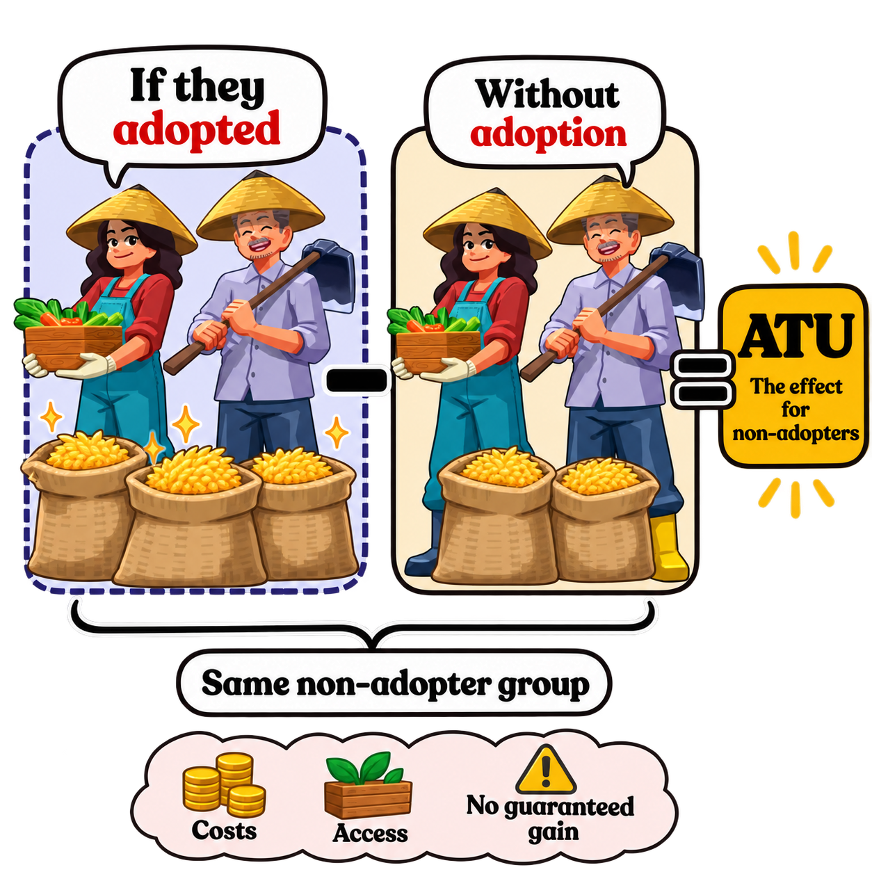
1.11 ATU: the effect for non-adopters
ATU means Average Treatment effect on the Untreated. Here, “untreated” means farmers who did not adopt.
The comparison stays with the same non-adopter group: their expected yield if they switched to the improved seed versus their expected yield without switching.
A positive ATU suggests that this group could achieve a higher average yield through adoption, under the model’s assumptions.
ATU answers: how much would adoption change the outcome for the group that did not adopt?
Costs, access, and feasibility still matter for an adoption recommendation.
1.12 Heterogeneity: differences between groups
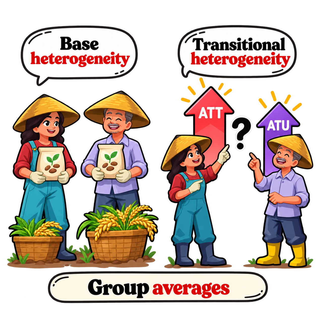
Base heterogeneity: imagine both groups using the same seed choice. Would their expected yields still differ because the groups themselves differ?
Transitional heterogeneity: would switching to the improved seed bring a larger average gain to current adopters or to current non-adopters?
A larger ATT than ATU suggests a greater estimated gain among current adopters. The reverse suggests a greater potential gain among non-adopters.
These are comparisons of group averages. They do not establish who benefits most individually.
Treatment and heterogeneity concepts: Di Falco, Veronesi, and Yesuf (2011).
1.13 What makes an ESR result credible?
- A clear definition of adoption and a suitable continuous outcome.
- Sensible explanatory variables and a defensible instrument choice.
- Enough information in both groups, with comparable characteristics where predictions are needed.
- A model that fits reliably, with uncertainty reported for its estimates.
The usual ESR model assumes a particular pattern for the hidden influences, called joint normality. This assumption helps it estimate the missing outcomes.
There is no single sample size or diagnostic result that guarantees a correct causal conclusion.

2 ESR in RAISINS
What the tables show and how to interpret the main metrics and tests
2.1 Where to find the results
Analysis Results contains the instrument checks, group comparisons, VIF, adoption model, and the two preliminary outcome models.
MLE & Treatment Effects contains the jointly estimated model, convergence information, selection test, and average treatment effects.
First understand the groups and instruments. Then check whether the model fitted reliably. Finally, read the treatment effects.
The following slides explain the tables in these two tabs.
2.2 Reading estimates and uncertainty
Estimate: what relationship does the model suggest, and how large is it? Read the sign alongside the variable’s units.
Standard error (SE): how precise is that estimate? A smaller SE relative to the estimate usually means less uncertainty.
t or z statistic: the estimate’s distance from the tested value, usually zero, relative to its uncertainty.
p-value: how surprising would evidence this strong be if the tested claim, usually “no relationship,” were true? A small value challenges that claim, but says little about practical importance.
A p-value is not the probability that the null hypothesis is true. “Statistically significant” usually means the p-value is below a chosen threshold such as 0.05. Lack of significance may reflect limited precision rather than absence of an effect.
2.3 Falsification Test of Instrument Validity
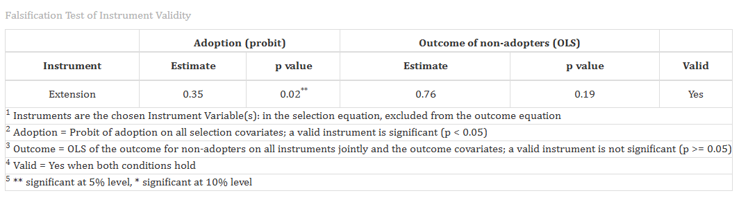
What it asks: does the instrument predict adoption, while showing no clear separate relationship with yield among non-adopters?
The table reports the instrument’s estimate and p-value in each check.
“Valid = Yes” means it meets the module’s screening rule. “No” means it does not meet that rule and needs investigation.
Treat this as an initial screen. The research setting must still explain why the instrument should not affect yield through another route.
The module’s rule requires an adoption p-value below 0.05 and a non-adopter outcome p-value at least 0.05. The latter regression includes the instruments jointly with outcome covariates. Conditioning on non-adoption can itself induce association through selection, and a non-significant result may reflect low precision.
2.4 IV diagnostics: weak instruments
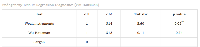
The IV Regression Diagnostics table uses an additional instrumental-variable model as a diagnostic check.
Weak instruments test: asks whether the instruments provide useful information about adoption after allowing for other predictors.
If an instrument tells us very little about who adopts, it gives the model little help in separating the adoption effect from other influences.
The common F above 10 guideline comes from linear IV practice. It is a rough warning threshold, not a guarantee that the ESR model is well identified.
2.5 IV diagnostics: Wu–Hausman and Sargan
Wu–Hausman: asks whether it is reasonable to treat adoption as unrelated to hidden influences on yield. A small p-value suggests that this would be questionable in the additional IV model.
Sargan: checks whether the additional instruments are consistent with the model’s assumptions about their relationship with the outcome. It generally needs at least two excluded instruments here.
A small Sargan p-value raises concerns about the instruments or model. A large p-value does not prove validity.
These are supporting checks. ESR has its own selection test in the MLE tab.
The auxiliary IV model treats adoption as a single endogenous regressor and uses a common adoption coefficient. It differs from ESR’s separate outcome equations. Wu–Hausman interpretation depends on valid instruments and the auxiliary model assumptions. See the ivreg package documentation.
2.6 Differences between adopters and non-adopters
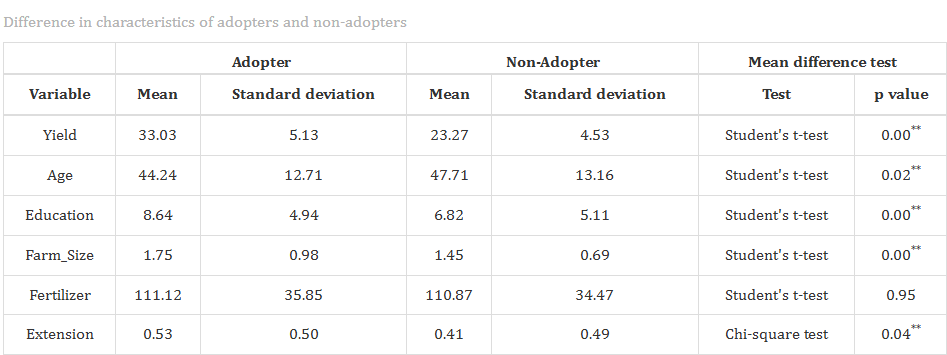
The Difference in characteristics table reports each group’s average and standard deviation.
- Mean: the group’s average value.
- Standard deviation (SD): how much individual values vary within the group.
- Comparison test and p-value: evidence that the groups differ on that characteristic.
RAISINS uses t-tests for continuous variables and a chi-square test for binary variables.
The table describes group differences. It does not show that adoption caused them.
For continuous variables, the module uses Levene’s test to assess differences in variance, then selects Student’s t-test or Welch’s t-test. These choices and test validity still depend on the data and their assumptions.
2.7 VIF: overlapping information in predictors
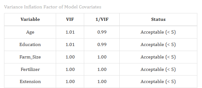
The Variance Inflation Factor table checks whether predictors contain strongly overlapping information.
For example, farm area recorded in two closely related measures may make their separate relationships with yield difficult to distinguish.
With larger VIF or smaller tolerance, the model has more difficulty separating the predictors’ individual relationships with the outcome.
The module’s reference values of 5 and 10 are guides for investigation. They are not automatic reasons to remove an important variable.
2.8 First Stage: Probit Selection Equation
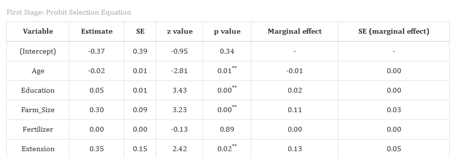
What it explains: which characteristics are associated with adoption.
A positive probit coefficient indicates a higher adoption tendency, holding other model variables fixed. A negative coefficient indicates a lower tendency.
Average marginal effects make the result easier to read: they express the relationship as a change in the probability of adoption.
For example, education’s marginal effect describes how adoption probability changes with another year of education, averaged across the sample.
A probit coefficient itself is not a percentage-point change.
For binary predictors, the module reports the average predicted probability change between the two categories. For continuous predictors, it averages the local marginal effect. An association in the selection model need not be a causal effect of the predictor.
2.9 First Stage: Model Fit Statistics
Null deviance: how well a basic model describes adoption before adding the explanatory variables. A larger deviance means poorer fit.
Residual deviance: the remaining lack of fit after adding those variables. A reduction means they help describe who adopts.
AIC: weighs improved fit against the cost of adding more parameters. Prefer a lower AIC when comparing suitable models using the same observations and outcome.
Degrees of freedom: information remaining after accounting for estimated parameters.
A better-fitting adoption model does not, by itself, establish a valid instrument.
2.10 Second Stage: Outcome Equations
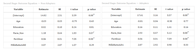
There is a coefficient table for non-adopters and another for adopters.
Each describes relationships between the chosen predictors and the outcome, with a selection correction term included.
For example, the fertilizer coefficient describes its association with yield within that model, allowing for the other predictors and selection correction.
A coefficient significant in one group but not the other does not automatically mean their coefficients differ.
These two-step results precede the full MLE estimates used for final interpretation.
2.11 Second Stage: Model Fit Statistics
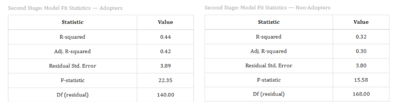
Each outcome model has its own fit table.
R-squared: how much of the observed variation the fitted equation explains. Adjusted R-squared also accounts for the number of predictors.
Residual standard error: the typical size of the unexplained outcome deviations, in the outcome’s units.
F-statistic: checks whether the slope terms collectively help explain the outcome.
A high R-squared does not establish that the estimated adoption effect is causal.
2.12 Sigma and rho: two different ideas
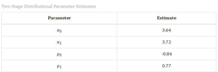
Sigma: how much do yields still vary beyond what the model explains? A larger sigma means more unexplained variation in that group.
Rho: how closely are hidden influences on adoption linked to hidden influences on yield in that regime?
Evidence that rho differs from zero supports the presence of unobserved selection. An imprecise estimate near zero does not prove selection is absent.
The Two-Stage Distributional Parameter Estimates are preliminary. Use the full MLE estimates for final interpretation.
The subscript 0 refers to non-adopters and 1 to adopters. Rho’s sign does not give the sign of ATT or ATU. Two-step rho estimates may fall outside the correlation range because the procedure does not constrain them. RAISINS warns about this and uses two-step values to initialize full MLE.
2.13 MLE: estimates and convergence
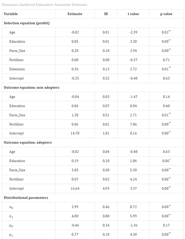
Parameter Estimates reports the adoption and outcome relationships estimated jointly, together with sigma and rho.
Convergence Diagnostics tells you whether the model-fitting procedure reached an acceptable stopping point. Read both the return code and message before relying on the estimates.
Log-likelihood is a measure of how well the model accounts for the data. There is no single value that means the model has “passed.”
Resolve convergence problems before interpreting treatment effects. Successful convergence still does not prove the model assumptions are correct.
2.14 Likelihood Ratio Test of Independence
What it asks: is there evidence that hidden influences on adoption are related to hidden influences on either outcome?
A small p-value provides evidence of such a connection within the ESR model.
A large p-value means the test found limited evidence of that connection. Selection may still be difficult to detect in the available data.
The LR test concerns selection. ATT and ATU concern the estimated outcome change due to adoption.
2.15 Average Treatment Effects: the outcome columns
Y1 is the expected outcome under adoption.
Y0 is the expected outcome under non-adoption.
Read across one group at a time. For adopters, Y0 answers “what if they had not adopted?” For non-adopters, Y1 answers “what if they had adopted?”
Both columns contain predicted outcomes, even when the treatment state matches the farmer’s actual choice.
The values in parentheses under Y1 and Y0 are SDs across household predictions, describing variation within the group.
2.16 Average Treatment Effects: effects and heterogeneity
The adopter row reports ATT. The non-adopter row reports ATU. Parentheses for treatment effects contain standard errors, describing uncertainty.
The ATH row compares the groups:
- Under Y1: base heterogeneity if both groups adopted.
- Under Y0: base heterogeneity if neither group adopted.
- Under treatment effect: transitional heterogeneity, comparing their average effects.
Read effect size, uncertainty, and units together. A positive effect is welcome for yield, but may be unwelcome if the outcome is production cost.
2.17 References
Lokshin, M., & Sajaia, Z. (2004). Maximum likelihood estimation of endogenous switching regression models. The Stata Journal, 4(3), 282–289. Article
Di Falco, S., Veronesi, M., & Yesuf, M. (2011). Does adaptation to climate change provide food security? A micro-perspective from Ethiopia. American Journal of Agricultural Economics, 93(3), 829–846. Article
Fox, J., Kleiber, C., & Zeileis, A. ivreg: Two-Stage Least-Squares Regression with Diagnostics. Documentation
Table names and interpretations were checked against the RAISINS ESR interface and server code. This guide distinguishes diagnostic screening rules from proof of causal identification. Standard ESR assumptions also include well-defined treatment, consistency, no interference, and exogenous outcome covariates. Selection correction does not solve all other forms of endogeneity.