Qualitative Data Analysis
Qualitative Data Analysis turns interview transcripts and other free text into codes, themes and simple summaries. This tutorial explains what coding a transcript means, how to create a project and add documents in RAISINS, how to build and organise a codebook, how to tag segments by hand or with the RA-One AI coder, and how to read the word-frequency, sentiment and codebook dashboards before exporting the finished project… Read more …
Qualitative Data Analysis (QDA) is used when the data are words rather than numbers, such as interview transcripts, open-ended survey answers, or field notes, and the goal is to organise that text into meaningful categories, called codes, and to summarise the patterns they reveal. RAISINS gives each study its own project, in which documents are added, a codebook is built, and passages of text are tagged with codes either by hand or with the help of the RA-One AI coder. It then reports word-frequency tables and clouds, lexicon- and LLM-based sentiment, and a codebook dashboard with a code matrix, heatmap, co-occurrence map and network, and exports the whole project as a single report, all without requiring you to write a single line of code. This tutorial walks through the module screen by screen, from logging in to the final export.
1 What is Qualitative Data Analysis?
Qualitative Data Analysis (QDA) involves examining non-numeric data like interview transcripts, open-ended survey responses, and field notes. You do this to identify, categorise, and interpret the meanings within the data. A key step in QDA is coding. Coding means attaching a short label, called a code, to a passage of text that expresses a specific idea. This allows you to retrieve and compare all passages that share the same idea later on. The complete list of codes, along with their definitions, is known as the codebook. You can also group related codes into broader categories called themes. After coding the text, you can summarise and report the patterns you find. This includes noting which ideas recur, in which documents they appear, and which other ideas they appear alongside.
Imagine a researcher is interviewing several paddy farmers to learn about the challenges they encounter. One farmer mentions unpredictable rain, another discusses the falling price of produce, and a third talks about the difficulty of hiring labour. When you read each interview separately, they seem like individual stories. However, if you label every mention of water as water management concern and every mention of price as market access concern, you can group all the water-related passages together and all the price-related passages together. This allows you to see which issue is mentioned most frequently across all the interviews.
How can the recurring ideas in a collection of interviews be found, organised, and summarised?
When you use QDA, it transforms your free text into a structured format by creating coded segments. In RAISINS, you have a workspace that helps you manage this process. You can store your documents and create a codebook, which is a list of codes you use to tag different parts of your text. Once you tag these segments, you can summarise the coded text. You can do this by analysing word frequencies, assessing sentiment, and using a codebook dashboard to view your results.
Qualitative Data Analysis (QDA) is different from methods that summarise data into a single number. Instead, QDA keeps the original words from interviews and organises them. When you use QDA, you assign a code to a specific part of the text. This code acts as a label. It helps you group together all passages with the same label so you can read and analyse them as a set. The codebook is a list that keeps track of all these labels and explains what each one represents.
2 Getting to the module
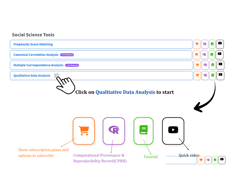
To open the module, first go to the RAISINS home page at www.raisins.live. Then, navigate to the Social Science Tools section. Click on Qualitative Data Analysis to begin.
In each module, you see four icons that link to different resources. The cart icon shows you information about subscriptions. The R icon takes you to the Computational Provenance & Reproducibility Record, which is explained later. The book icon opens this tutorial for you to read. The play button starts a video walkthrough.
2.1 Computational Provenance & Reproducibility Record
The CPRR (Computational Provenance & Reproducibility Record) gives you a clear and detailed account of your analysis process. When you click the CPRR icon on the module’s landing card, you see the exact computational workflow for each result. This record includes the R version and the exact version of every package used. It also names the specific function responsible for each output, such as word-frequency tabulation and sentiment scoring with each lexicon. Additionally, it covers the codebook, matrix, and network summaries. The record lists every default parameter and decision rule the module applies. It also provides fully runnable R code for each step, allowing you to verify results independently. The record has its own DOI, ensuring it is uniquely identifiable.
When you need to cite the platform in a paper, thesis, or report, use the RAISINS citation. You can find it in APA, Harvard, and BibTeX formats at www.raisins.live/citation.html. This citation serves as the main reference, and it is usually sufficient for most manuscripts.
The CPRR for the Qualitative Data Analysis module is at www.raisins.live/module_record/qda.html.
Use the RAISINS paper as your main reference when discussing the platform. Include the CPRR as additional documentation if a journal requests specifics about the computing environment. This is also useful if you want your methods section to specify exact versions and functions, instead of just stating “analysis was carried out using an online tool.”
3 The Welcome page: preview and logging in
When you open the module, you start on the Welcome page (Figure 2). Here, you can explore the module using Preview mode. This mode lets you look at a built-in demonstration project. You can see all the features like coding, word frequency, sentiment analysis, and the codebook dashboard. However, you cannot create your own project in this mode. If you want to work with your own data, you have two options at the bottom of the card. Click Get Started for an individual subscription or Institutional Login if you have access through a subscribing institution. The card also provides links to Subscribe, watch a Quick video, Contact Us, and view the licence and version information.
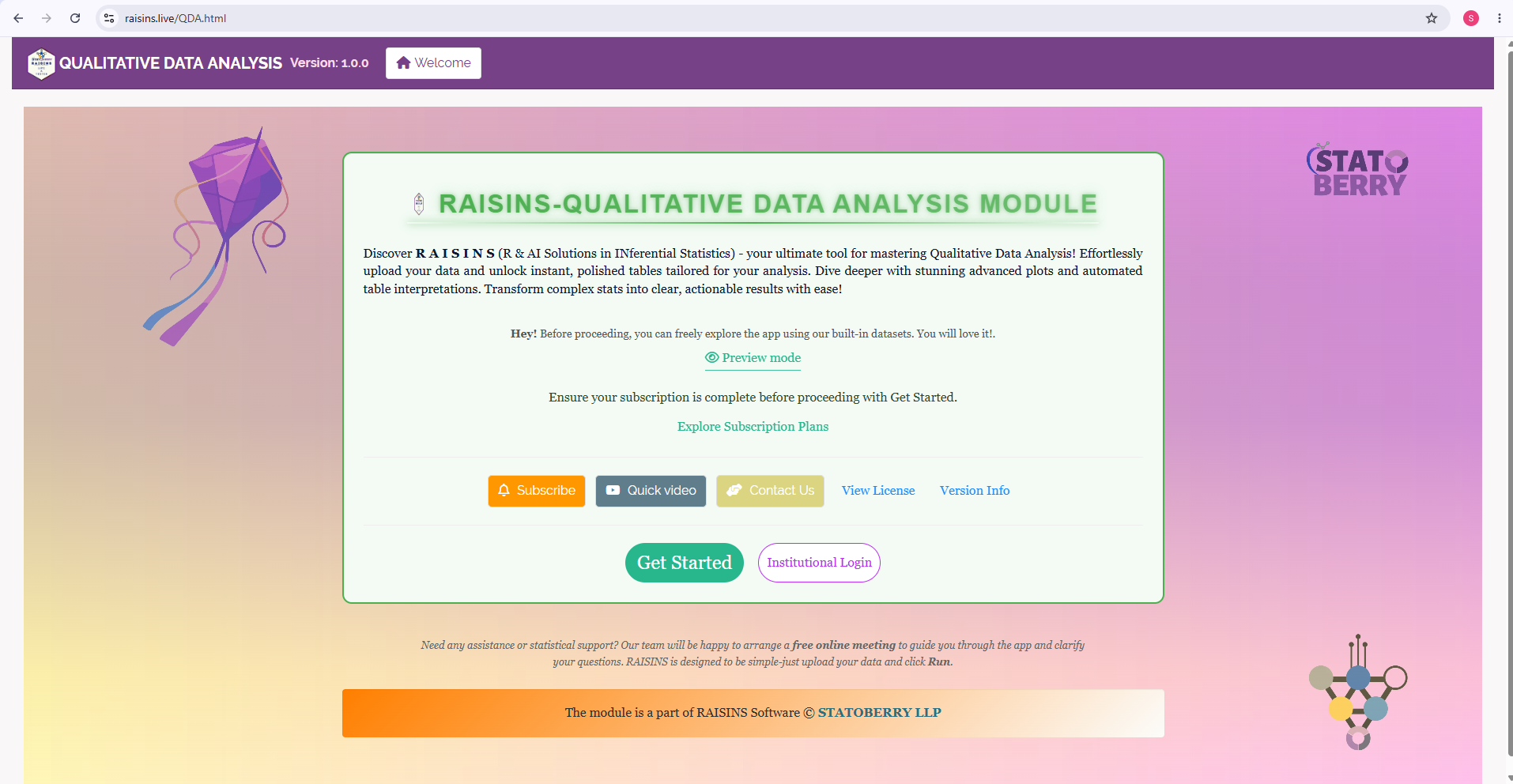
When you are in preview mode, you can only view the demonstration project. You cannot make any changes or create new projects. To start your own projects, add documents, and save your coding work, you need to sign in. You can do this by clicking on Get Started or using Institutional Login. Once signed in, you can access all the features described from Section 5 onward.
4 A working example
In the rest of this tutorial, you will work with a project called the Demo interview project. This project includes two interview transcripts, labelled interview_farmer_01.txt and interview_farmer_02.txt. These transcripts capture conversations with farmers about paddy cultivation in the Alappuzha district. The discussions cover topics such as the challenges farmers encounter, changes in yield and price, labour issues, and the support they receive. Each transcript is a straightforward text of a conversation between an interviewer and a farmer.
In this tutorial, you will see the project being coded in real-time. As we progress, the codebook and the segment counts will increase. This project is the same one you can access in Preview mode. This means you can replicate every screen and step exactly as shown.
To get started, open the module in Preview mode (Section 3). Then, open the Demo interview project. This project contains all the figures used in this tutorial. By using it, you can follow along with each step without needing to create any files yourself.
5 My Projects: creating and editing a project
Once you sign in, you will see the My Projects page (Figure 3). This is where all your studies are organised as separate projects. Each project is displayed as a card. Next to these, you will find a dashed New project card. This card indicates how many more projects you can create based on your subscription. If you need help navigating the page, there is a Take a tour link at the top right. Clicking this link will replay a short guided walkthrough of the page whenever you need it.
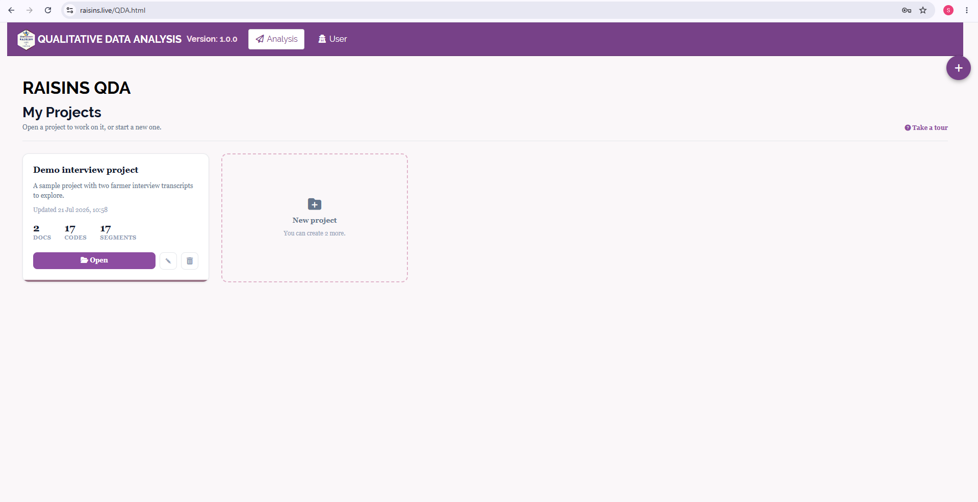
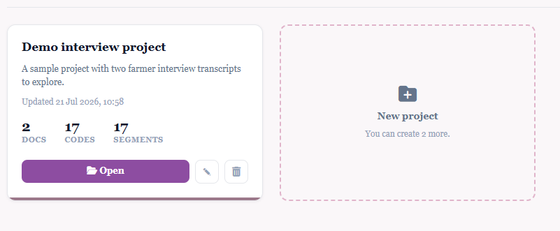
A project card gives you a quick overview of your project. It shows the project’s title, description, the date it was last updated, and the counts of documents, codes, and segments. Below this information, you will find three controls (Figure 4). The Open button takes you into the project workspace (Section 6). The pencil icon lets you edit the project’s name and description. The trash icon allows you to delete the project. The counts displayed on the card represent the project’s last saved state. This means they might not match the current counts you see while the codebook is being rebuilt in Section 11.
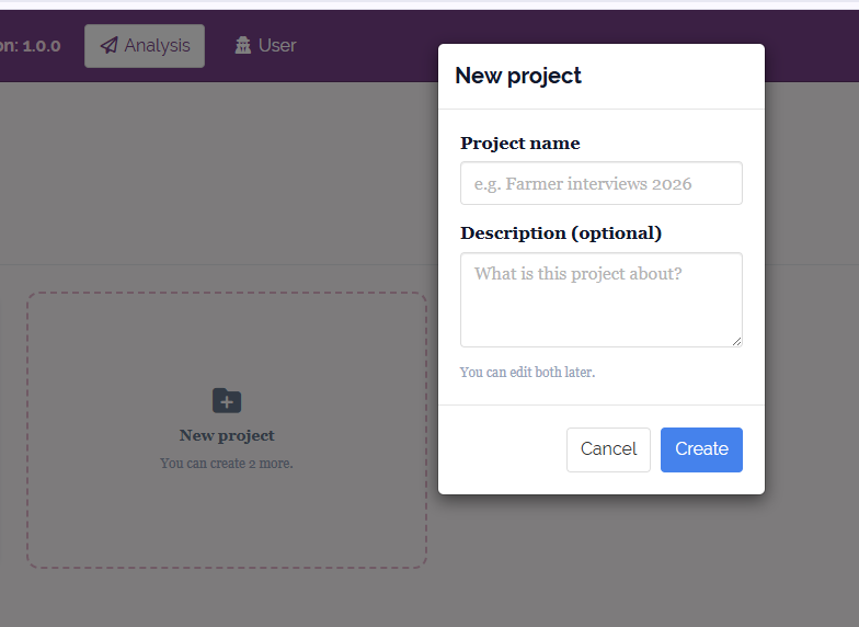
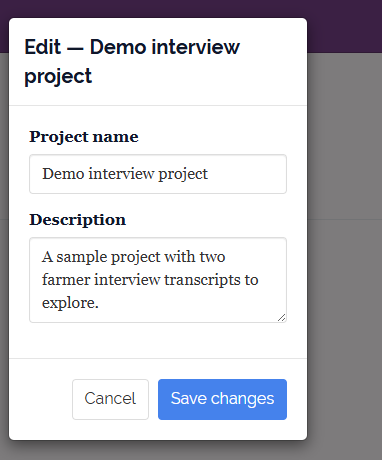
To begin a new study, you need to click on the New project card. A dialog box will appear, asking you to enter a Project name and, if you wish, a Description (Figure 5 (a)). Don’t worry if you’re unsure about these details right now; you can change them later. Once you’ve entered the information, click Create. This action will add a new, empty project and open it for you to start working. If you want to change the name or description of an existing project, click the pencil icon on the project’s card. This will open the fields with the current information already filled in (Figure 5 (b)). After making your changes, click Save changes to update the project details.
6 Opening a project and adding documents
When you click Open on a card, you enter the project workspace (Figure 6). At the top, you will see a row of tabs: Project, Codebook, Word Frequency, Sentiment, Export, and FAQs. These tabs help organise the module, and this tutorial will guide you through them in order. Start with the Project tab, where you will perform the coding tasks. Within the Project tab, there are sub-tabs: Transcript, Keyword in Context, Tagged Segments, and RA-One coder. On the left side, there is a rail that allows you to switch between the Documents list and the Codebook.
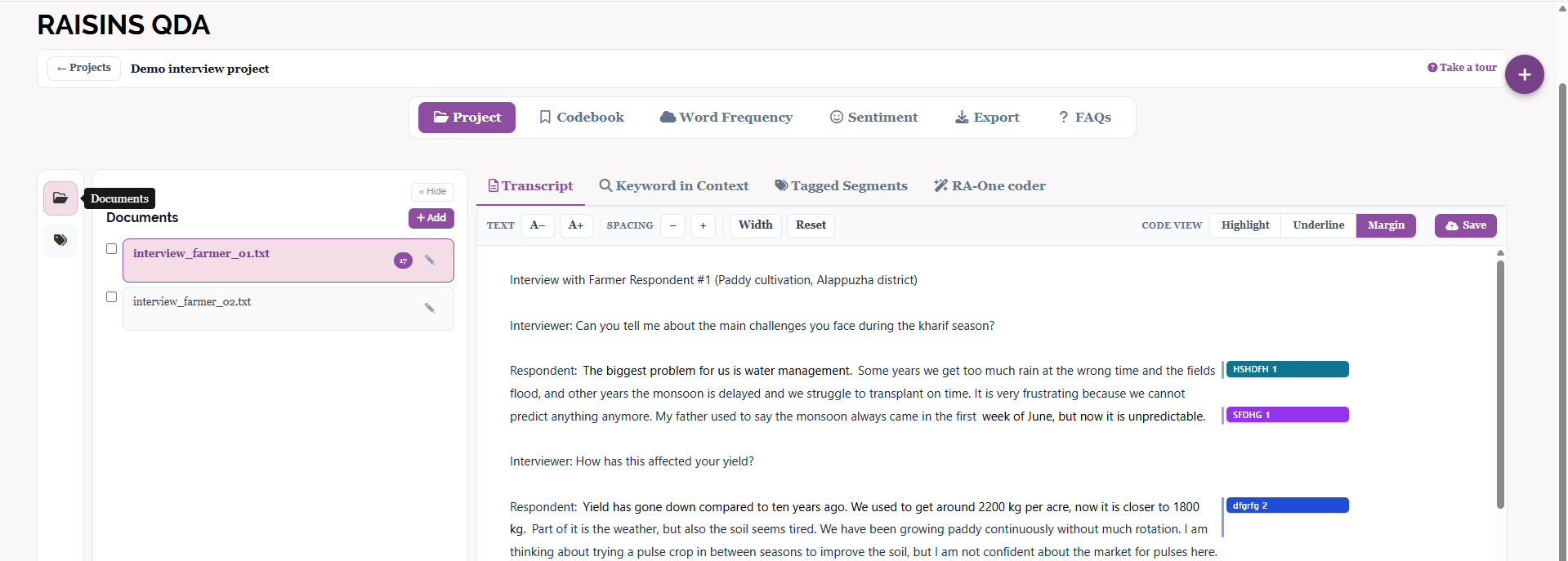
In the Documents rail, you will find a list of all the transcripts in your project. You can select any transcript from this list to read it in the Transcript panel. If you want to add a new transcript, click on + Add at the top of the rail. Then, provide the document you wish to include. Once added, the new transcript will appear in the list, ready for you to open and code. Your project can contain multiple documents. The analysis tabs allow you to choose which documents to include or exclude from your analysis.
At the top of the transcript, you will see a small toolbar. The TEXT option with (A− / A+) lets you change the size of the text you are reading. The SPACING option allows you to adjust the space between lines. Width and Reset help you control the width of the column you are viewing. The Save button is used to store your coding work. The CODE VIEW switch offers different ways to display coded passages: Highlight, Underline, or Margin. More details about this feature are provided in Section 8.
7 Building your codebook: adding and editing codes
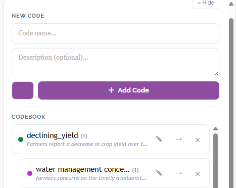
Switch the left rail to the Codebook to manage codes. At the top is a New Code form (Figure 7 (a)) with a Code name, an optional Description, and a colour swatch that sets the colour the code’s highlights and labels will use in the transcript. Type a name, choose a colour, and click Add Code. Until the first code is added, the codebook reads “No codes yet; add your first code above.”
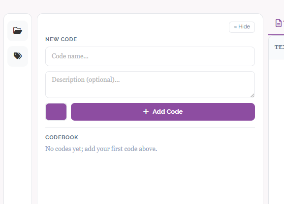
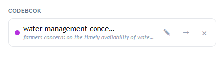
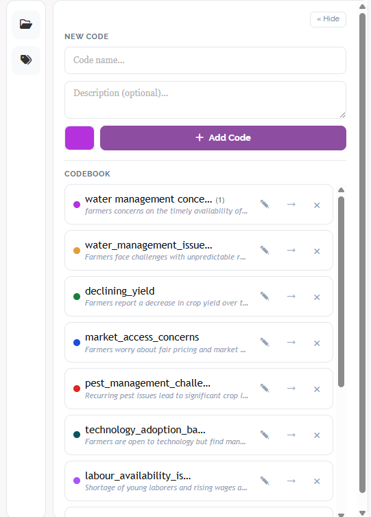
Each saved code appears in the codebook list with its colour dot and, in brackets, the number of segments tagged with it (Figure 8). Three controls sit beside every code: a pencil to edit it, an arrow (→) to promote or move it, and an × to remove it. As coding proceeds, this rail becomes the working list of codes you tag from.
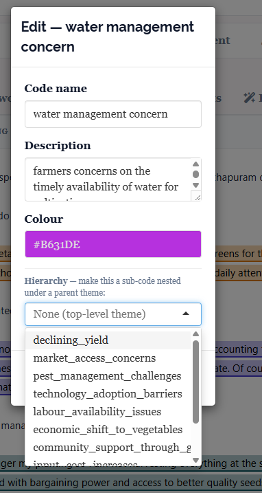
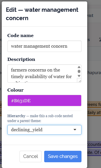
Clicking the pencil opens the Edit dialog (Figure 9 (a)), where the name, description and colour can be changed. The dialog also carries a Hierarchy dropdown, “make this a sub-code nested under a parent theme”, which lists the other codes as possible parents. Choosing a parent (Figure 9 (b)) and clicking Save changes nests the code beneath it, so that specific codes can be organised under broader themes. In the working example, water management concern is nested under declining_yield, and the rail then shows it indented as a sub-code (Figure 10).
You do not need a finished codebook before you start coding. Add a code the moment you meet an idea worth labelling, refine its name or colour later through the pencil, and group related codes into themes with the Hierarchy dropdown once the broad patterns become clear.
8 Tagging segments in the transcript
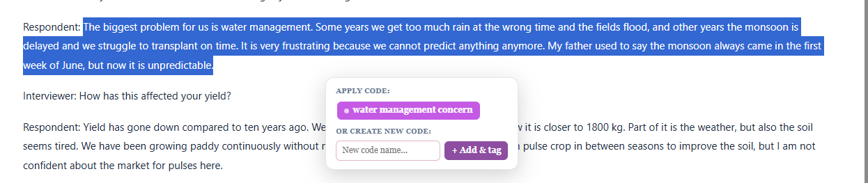
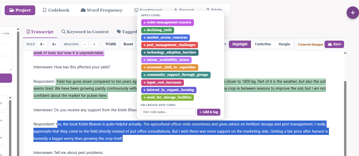
Coding a passage is done directly in the Transcript panel. Select the text you want to code with the cursor, and an Apply Code popover appears at the selection (Figure 11 (a)). It lists the existing codes as coloured buttons; clicking one tags the selected passage with that code. The popover also offers or create new code, a name field with an + Add & tag button that creates a brand-new code and applies it to the selection in a single step (Figure 11 (b)). A tagged passage is called a segment.
How coded segments are shown is set by the CODE VIEW switch in the toolbar, which offers three styles (Figure 12). Highlight fills the passage with the code’s colour, Underline draws a coloured line beneath it, and Margin leaves the text plain and places a coloured code label in the right margin beside it. The three views show the same coding in different ways; choose whichever keeps a densely coded transcript readable. Remember to click Save in the toolbar; the toolbar shows Unsaved changes until you do, and the time of the last save afterwards.
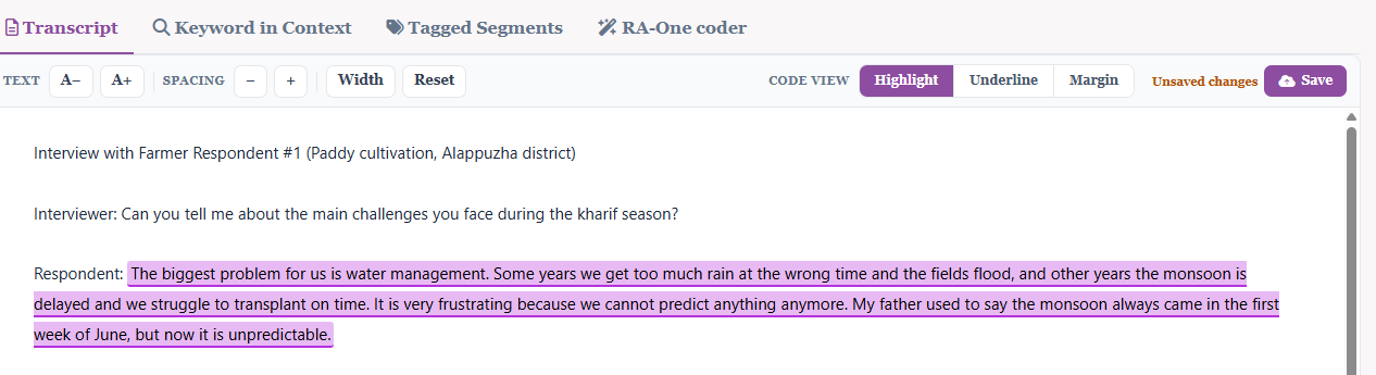
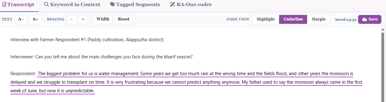
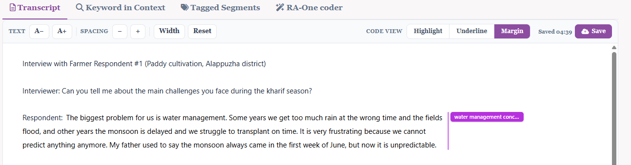
Coding is stored only when you click Save. While the toolbar reads Unsaved changes, your most recent tags exist only in the browser; navigating away without saving can lose them. Save whenever the indicator changes, and confirm it reads a recent save time before moving on.
9 Reviewing coded work: Tagged Segments and Keyword in Context
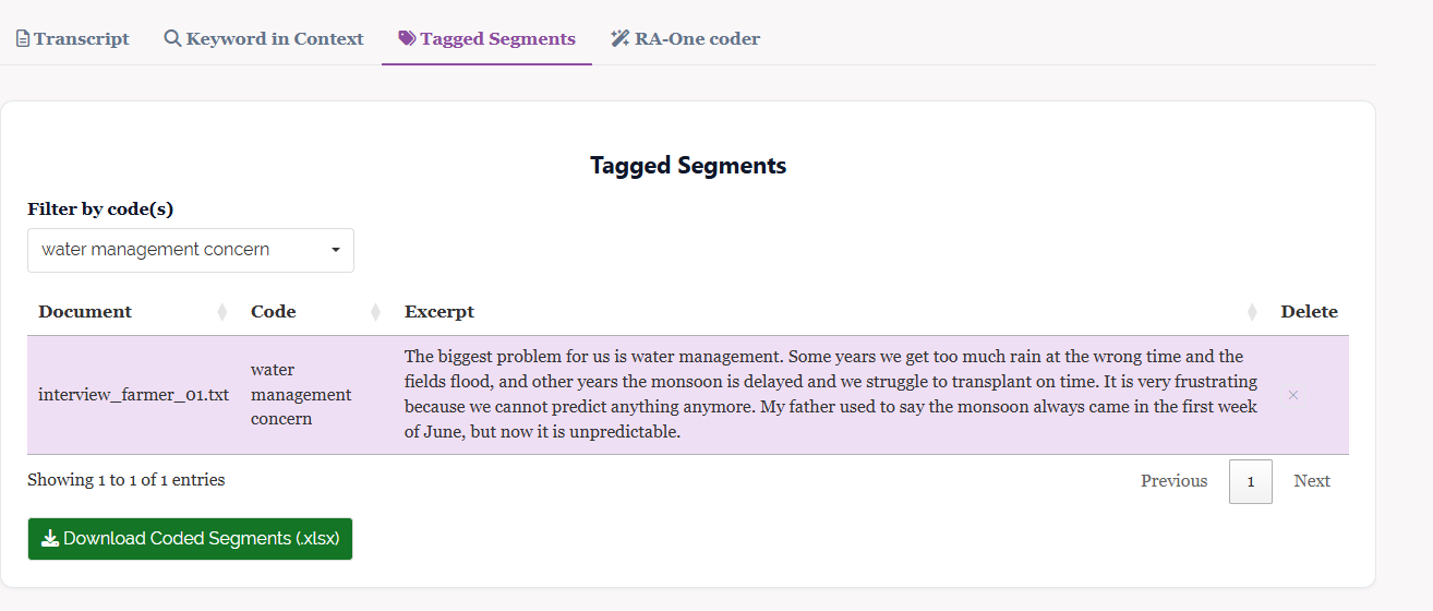
Two further sub-tabs of the Project tab help you review and search the coding. Tagged Segments (Figure 13) gathers every coded passage into one table, with the document it came from, the code applied, and the excerpt itself. A Filter by code(s) control at the top narrows the table to one or more codes, so all passages sharing an idea can be read together, exactly the retrieval that coding makes possible. Each row has an × to remove that tag, and Download Coded Segments (.xlsx) exports the whole table.
Keyword in Context (KWIC) (Figure 14) searches the raw text rather than the codes. Enter a Search term, choose which documents to search, and click Search; each occurrence is listed with a line of surrounding context and the document it appears in. In the working example, searching “Mechanization” returns one match in interview_farmer_01.txt. A Move to section button jumps from a result straight to that point in the transcript, so a passage worth coding can be found and tagged quickly, and Download Results (CSV) saves the matches.
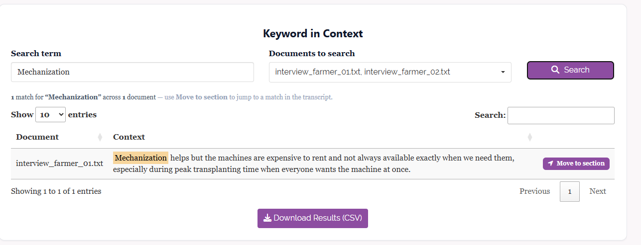
Use Tagged Segments to review what you have already coded, all excerpts for a code, side by side. Use Keyword in Context to explore text you may not have coded yet, locating every mention of a word so you can decide what deserves a code.
10 RA-One coder: AI-assisted coding
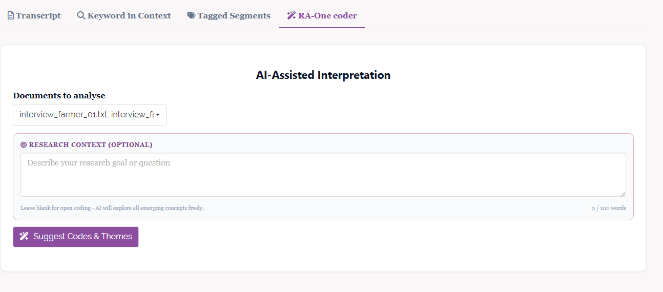
The RA-One coder sub-tab offers AI-assisted coding for when you would rather start from a suggested set of codes than build one from a blank page. Choose the documents to analyse and, optionally, describe your research context, the goal or question guiding the study (Figure 15). Leaving the context blank invites open coding, in which RA-One proposes whatever concepts emerge from the text; filling it in focuses the suggestions on your stated question. Click Suggest Codes & Themes to run the analysis.
RA-One returns a list of suggested codes (Figure 16), each with a short definition and a representative quote drawn from the text, for instance water_management_issues, declining_yield, market_access_concerns, and pest_management_challenges. Tick the codes you want, or use Select all, and click Add Selected to Codebook; they are added to the codebook (Section 7) with colours already assigned, ready to be applied to segments like any hand-made code. The suggestions are a starting point to review and edit, not a finished analysis.
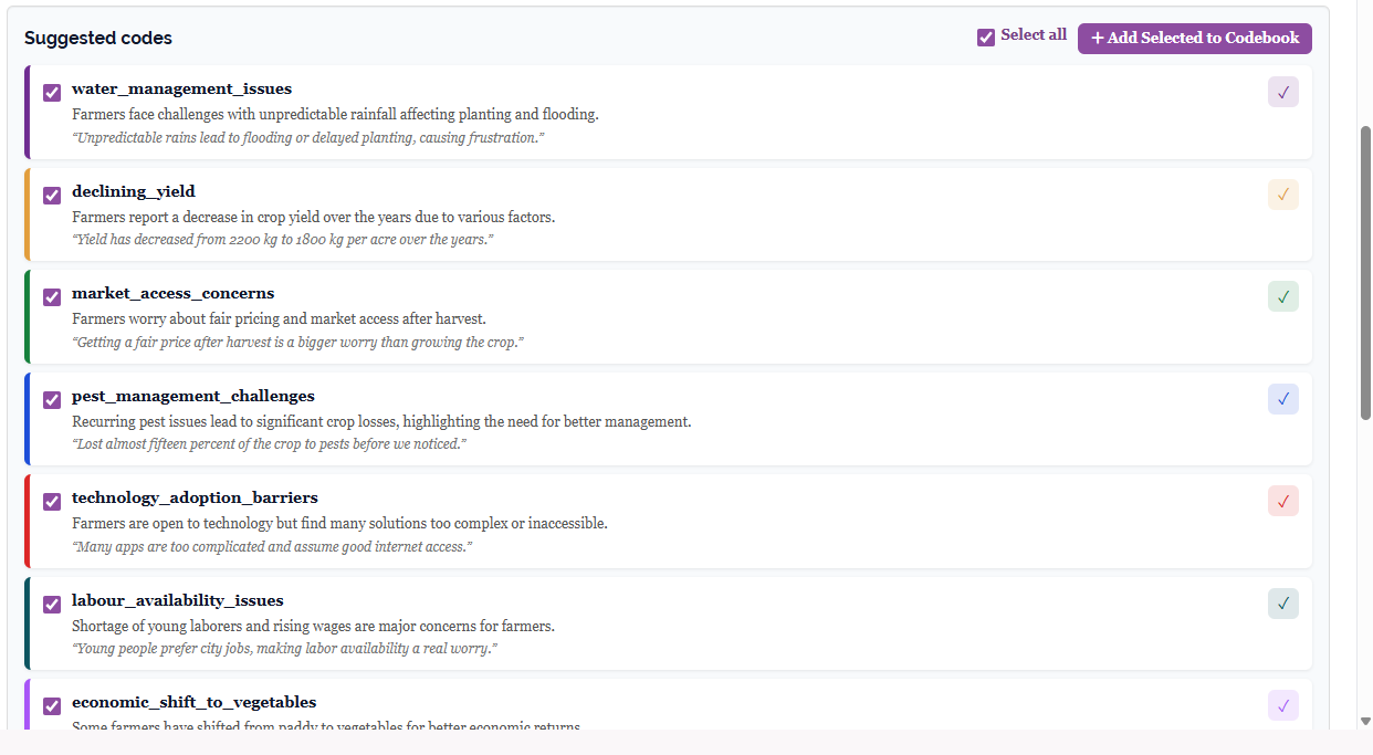
RA-One reads the transcripts and proposes codes, but the decision of which codes are meaningful for your study remains yours. Treat the list as a fast first draft of the codebook: keep the codes that fit, rename or discard the rest, and always check each suggested code against the passages it is meant to describe.
11 The Codebook dashboard
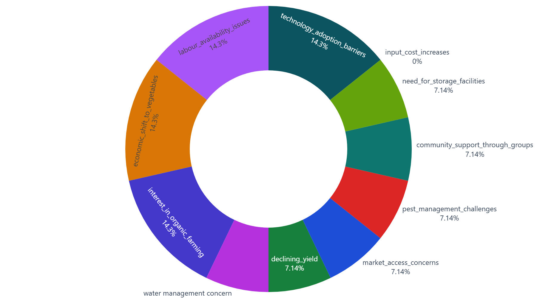
The Codebook tab summarises the coding across the whole project. Four tiles at the top report the totals, in the working example 11 codes, 14 coded segments, 2 documents, and an average of 1.3 segments per code (Figure 17). Beneath them, the Codes list ranks each code by how many segments carry it, and the Codebook visualisation on the right redraws that information in five views, selected by the toggle: code frequency, by document, co-occurrence, share, and hierarchy. Download Codebook Summary (.xlsx) exports the underlying counts.
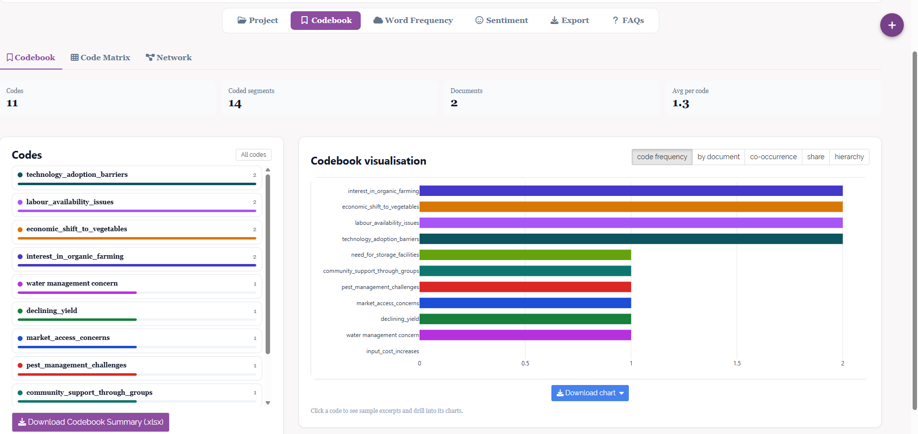
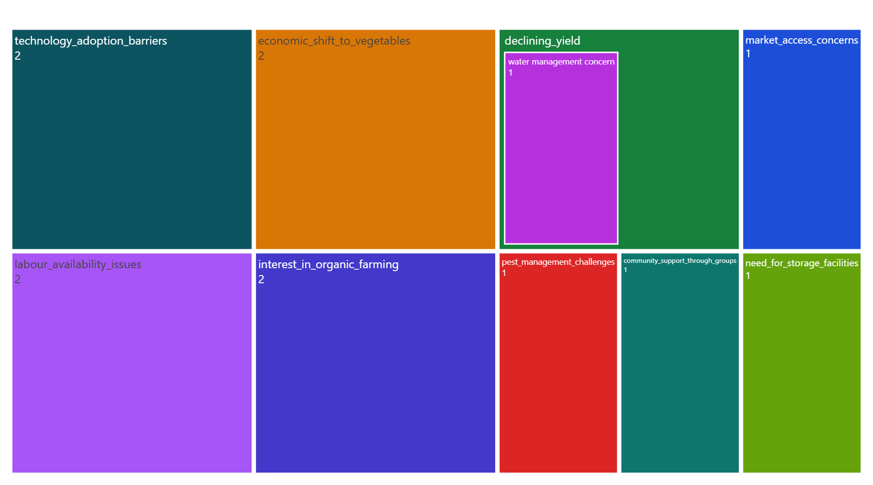
The code frequency view is a simple bar chart of segments per code; here four codes, interest_in_organic_farming, economic_shift_to_vegetables, labour_availability_issues and technology_adoption_barriers, lead with 2 segments each, most others have 1, and input_cost_increases has none. The share view (Figure 18 (a)) shows the same counts as percentages of all coded segments, and the hierarchy view (Figure 18 (b)) draws the codebook as nested boxes, so a sub-code such as water management concern appears inside its parent theme declining_yield, exactly the nesting set in Section 7.
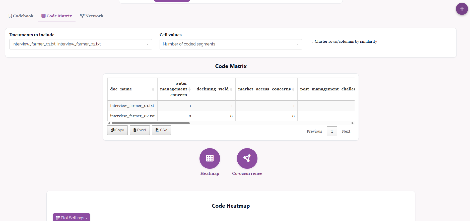
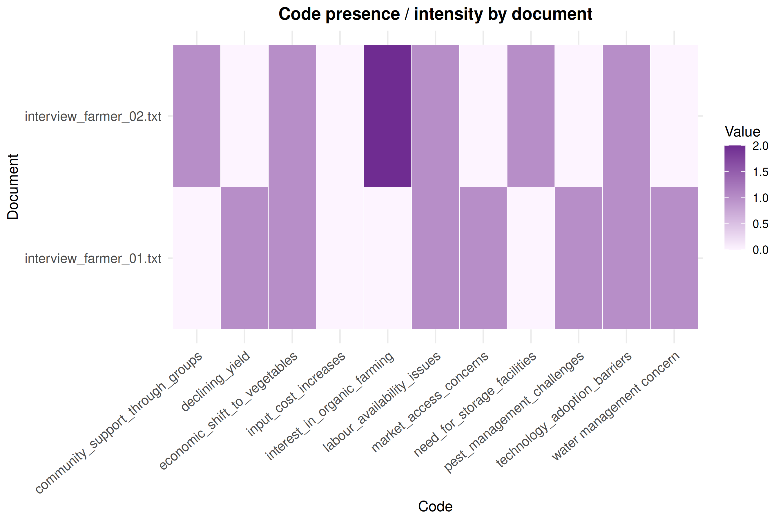
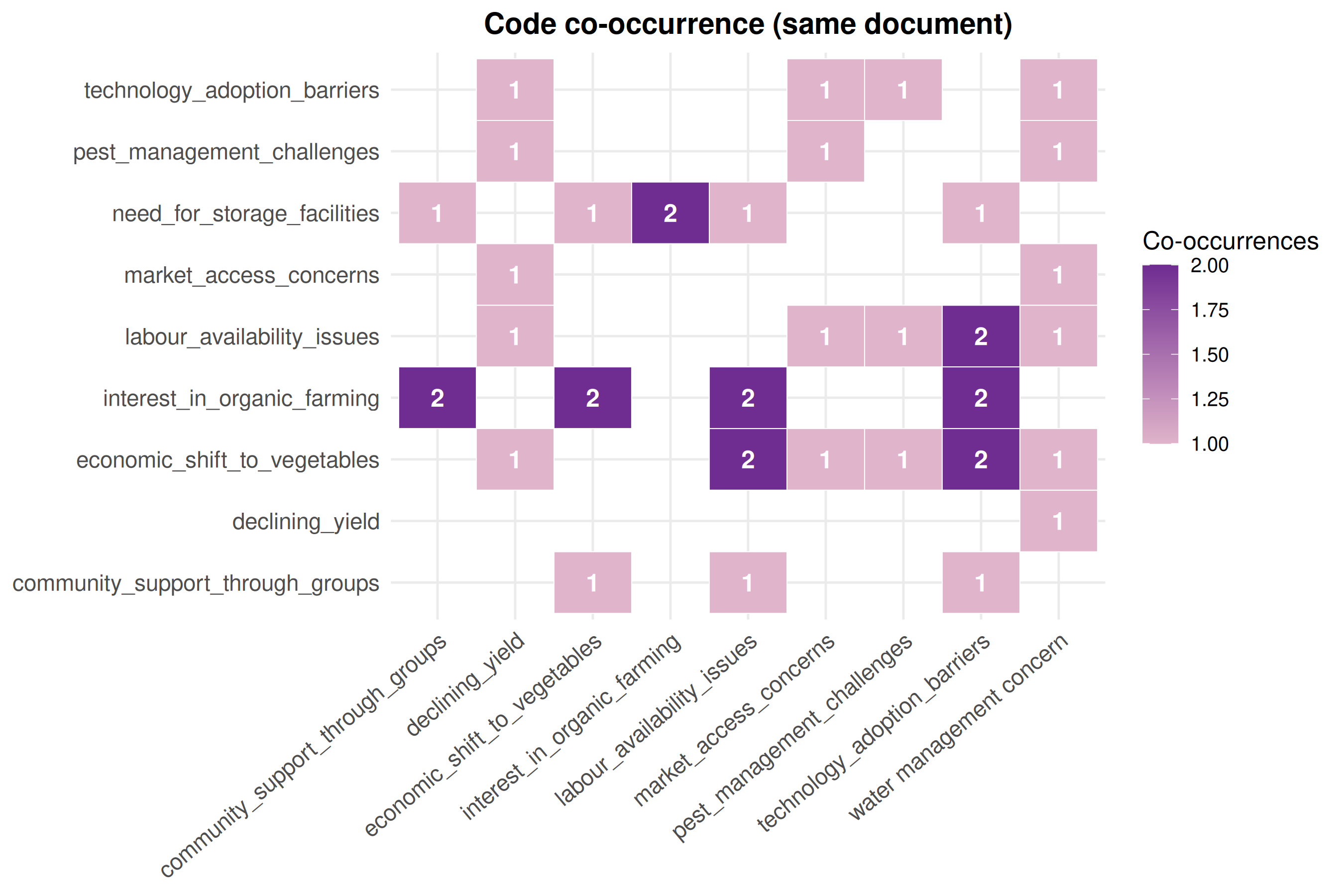
The Code Matrix sub-tab crosses codes against documents (Figure 19). With Cell values set to Number of coded segments, each cell reports how many segments in a given document carry a given code; in the working example the first three codes appear once each in interview_farmer_01.txt and not at all in interview_farmer_02.txt. An option to cluster rows/columns by similarity groups documents and codes that pattern alike, and the table can be copied or exported to Excel or CSV. Two icons below it redraw the matrix as a Heatmap (Figure 20 (a)), shading each document–code cell by intensity, and as a Co-occurrence map (Figure 20 (b)), counting how often each pair of codes appears together in the same document.
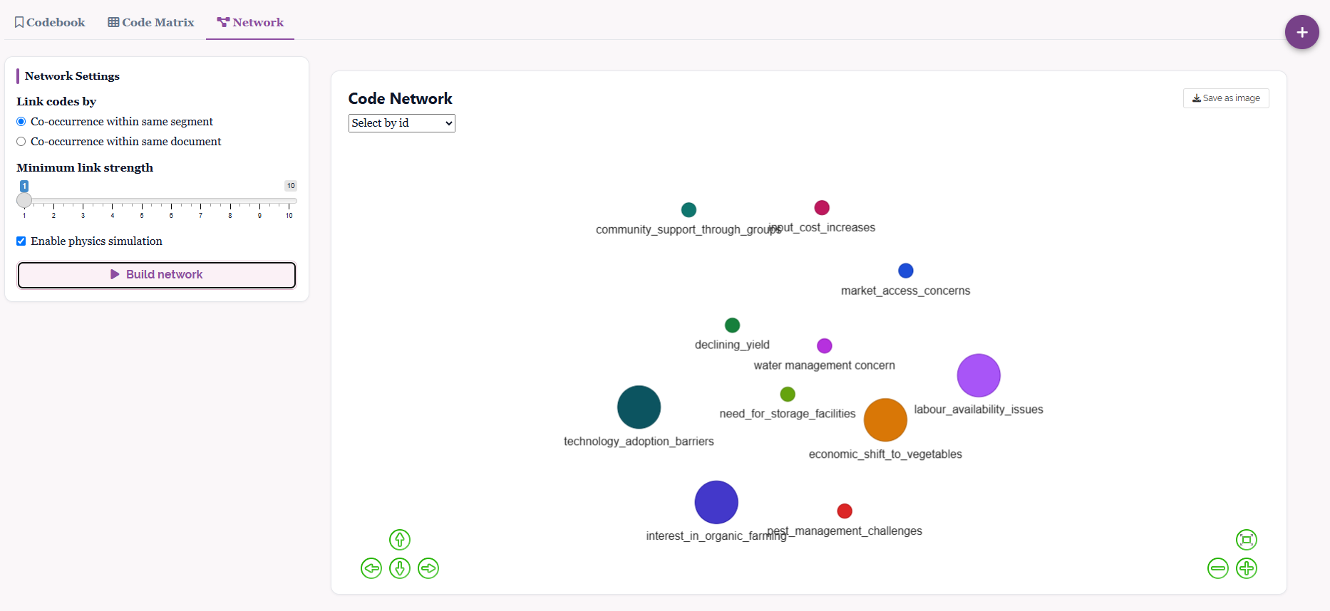
The Network sub-tab draws the codes as a graph (Figure 21). Under Network Settings, codes can be linked when they co-occur within the same segment or within the same document, a minimum link strength slider hides weaker links, and a physics simulation spreads the nodes out. Each node is a code, sized by how often it is used, and each line joins codes that occur together, giving a map of which ideas travel together across the interviews. Build network redraws it and Save as image exports it.
A code used more often is not automatically more important; it may simply describe a common turn of phrase. Read the dashboard alongside the actual segments in Section 9: the counts show where to look, but the passages themselves tell you whether a frequent code is substantively meaningful or merely repetitive.
12 Word Frequency
The Word Frequency tab counts the words in the selected documents and reports them in a Frequency Table giving each word, its count, and its relative frequency as a percentage (Figure 22). A Filters panel controls the count: the number of words to display, a minimum word length (skip words shorter than), group similar words (lemmatise), which counts farm and farms together, and ignore common words, which removes function words such as the and is. An also ignore these words box lets you add your own stop-words.
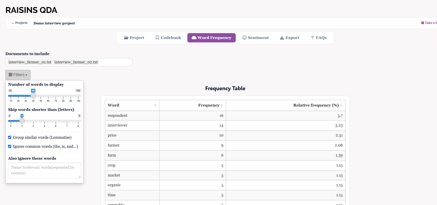
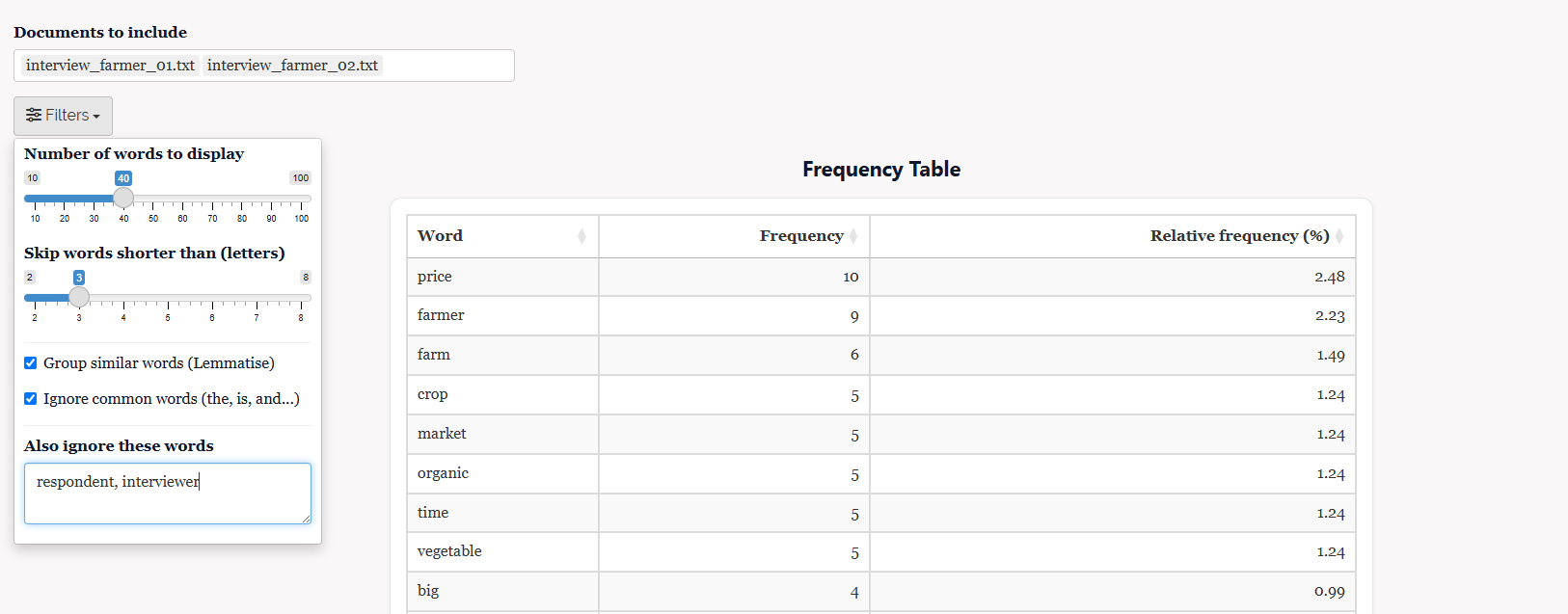
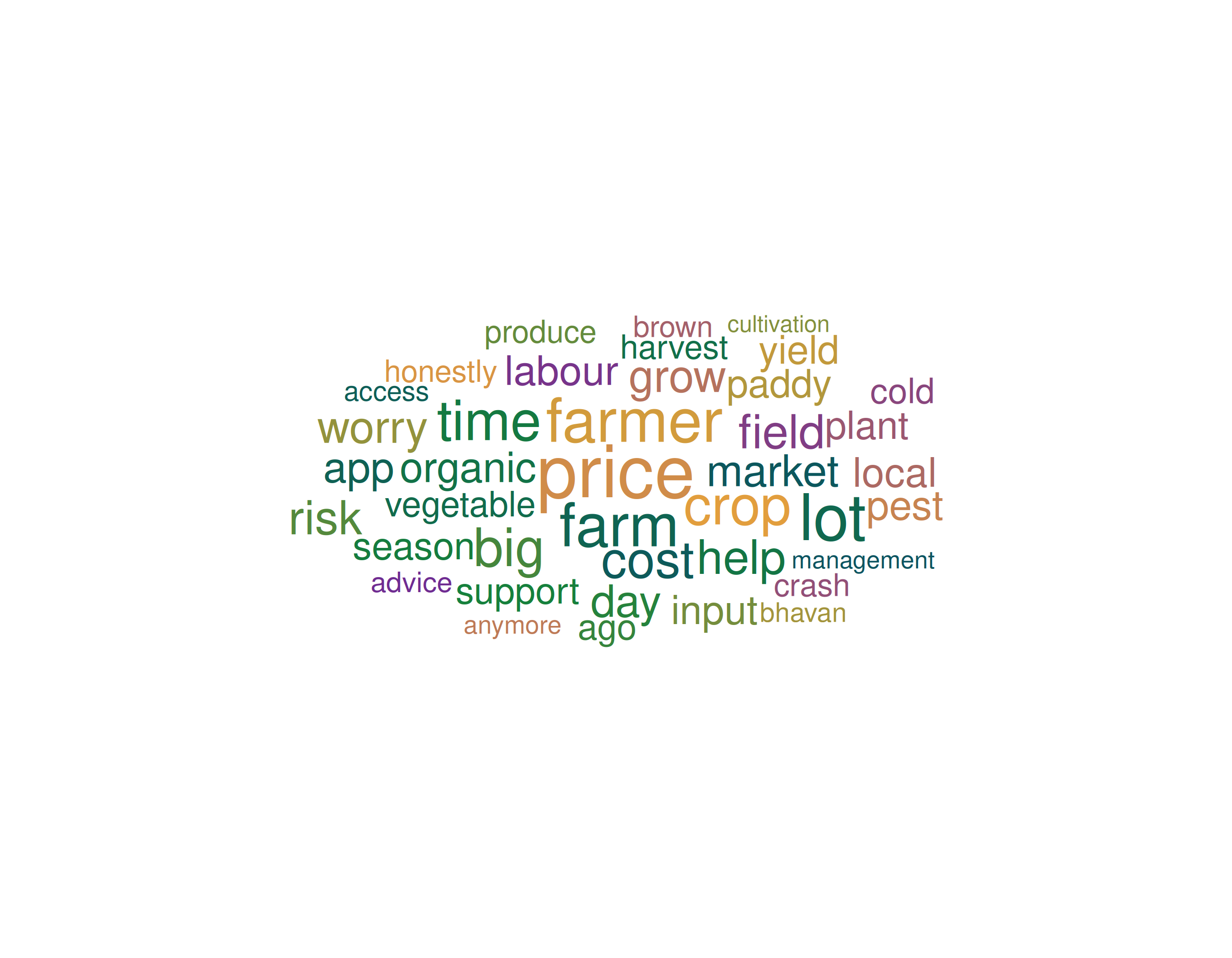
Without custom stop-words, the most frequent terms in the working example are the interview scaffolding, respondent (16) and interviewer (14), followed by price (10) and farmer (9). These structural words rarely carry meaning, so adding respondent, interviewer to the ignore box removes them and lifts the content words to the top: price (10, 2.48%), farmer (9), farm (6), then crop, market, organic, time and vegetable at 5 each (Figure 23). The recurring prominence of price and market echoes the market-access concerns seen in the coding.
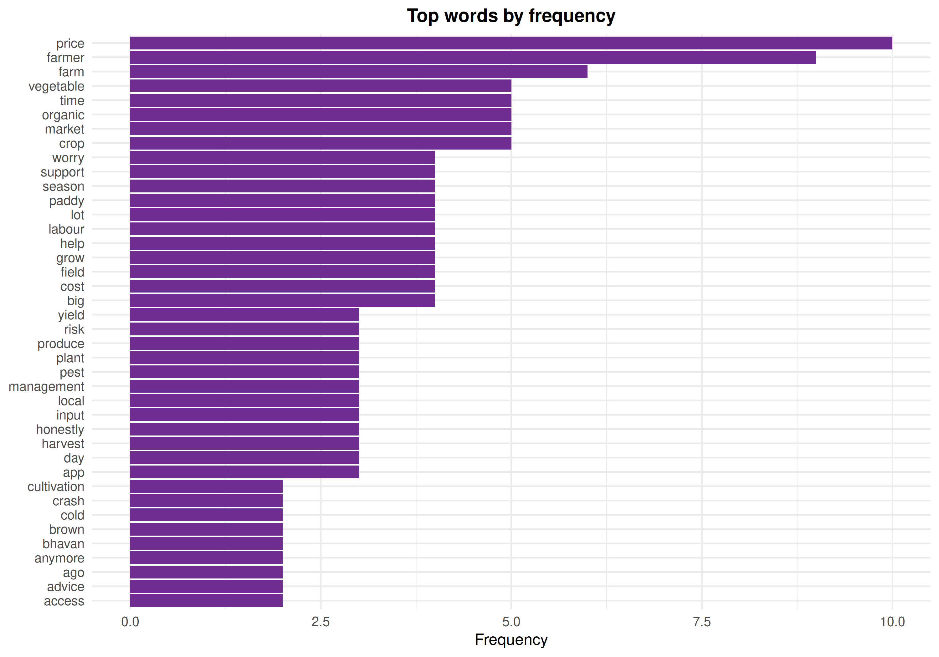
The same counts can be downloaded as a bar chart of the top words (Figure 24 (a)) or as a word cloud in which size is proportional to frequency (Figure 24 (b)). Both are visual restatements of the frequency table, useful for a report or a quick overview.
A high count shows that a word is common, not that it is important; interview scaffolding and filler words are often the most frequent of all. Use the stop-word filter and lemmatisation to clear these away, and read the surviving high-frequency words as prompts for closer coding rather than as conclusions in themselves.
13 Sentiment analysis
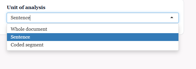
The Sentiment tab estimates the emotional tone of the text (Figure 25). Three controls set it up: the documents to include, the method used to score words, and the unit of analysis. The method dropdown offers four lexicon approaches, Bing, NRC Emotion, AFINN, and VADER, and one LLM-based option, RA-One Sentiment (Figure 26 (a)); the unit of analysis dropdown scores by whole document, sentence, or coded segment (Figure 26 (b)). A lexicon method matches words against a fixed dictionary of sentiment terms, while the RA-One option reads each unit in context.
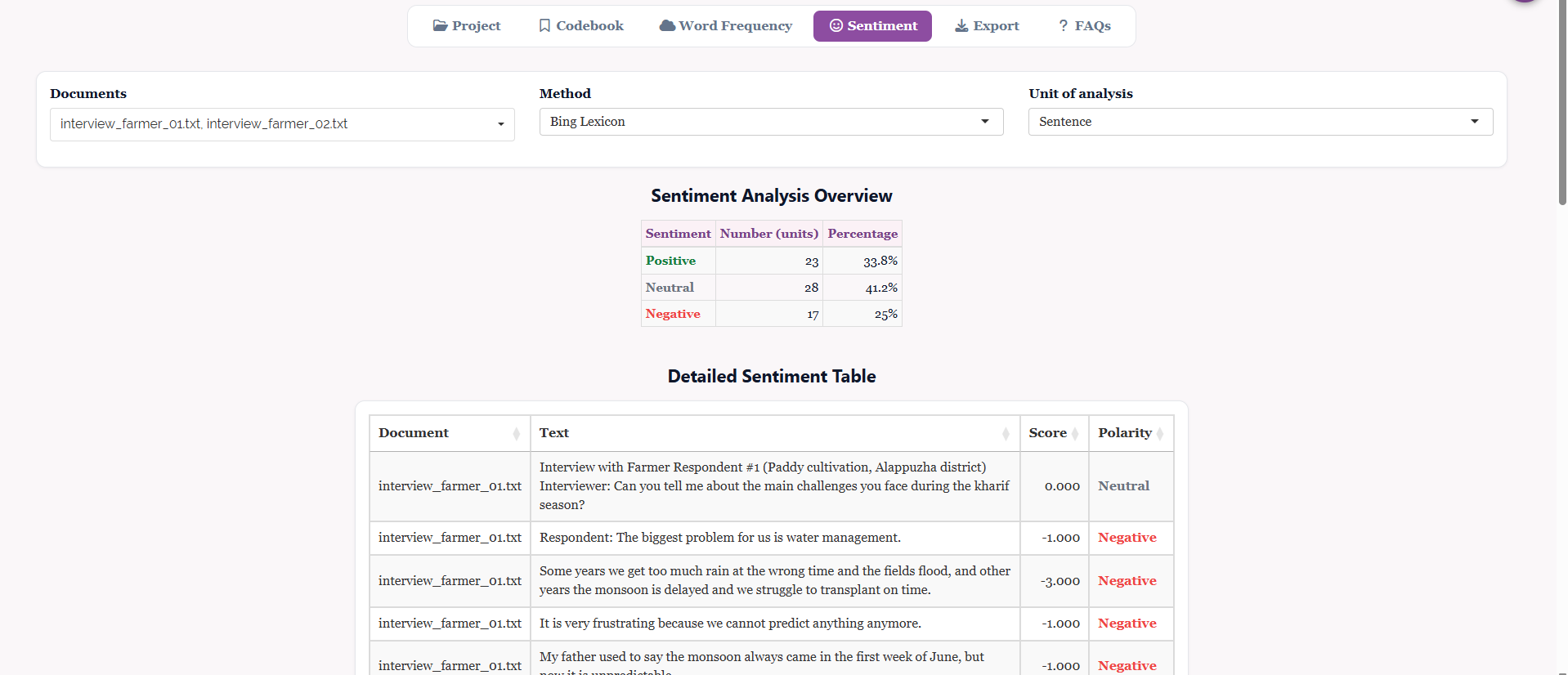

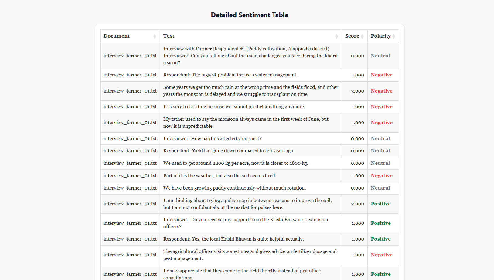
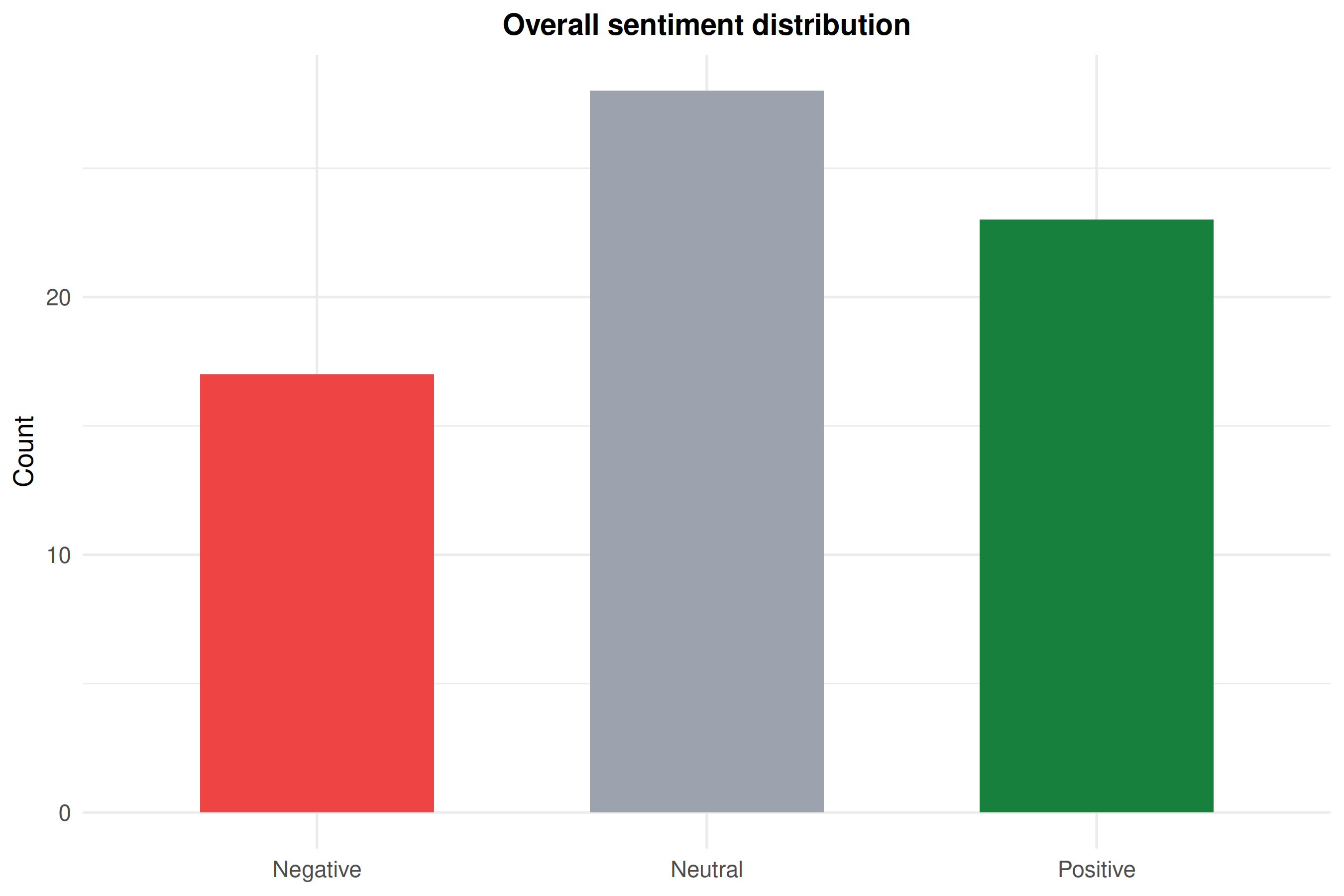
The Sentiment Analysis Overview counts how many units fall into each class. In the working example, scored by sentence with the Bing lexicon, 28 sentences (41.2%) are neutral, 23 (33.8%) positive, and 17 (25%) negative, a mixed but slightly positive picture. The Detailed Sentiment Table (Figure 27) lists every unit with its score and polarity, so the classification can be checked sentence by sentence; the opening line about water management, for instance, scores −3 and is flagged negative, while the remarks about local support score positive.
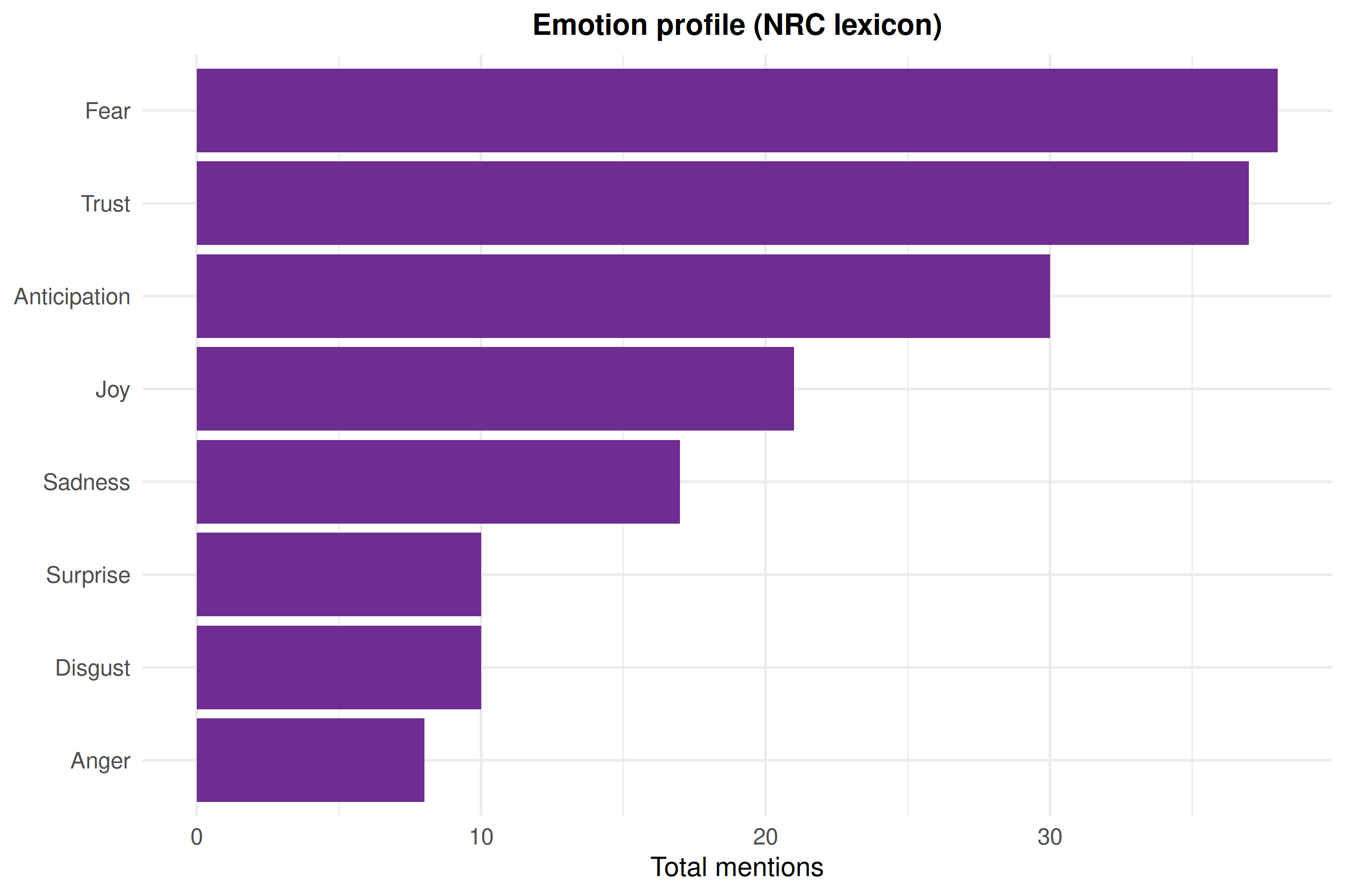
Two charts summarise the result: the overall sentiment distribution (Figure 28 (a)), a bar chart of the positive, neutral and negative counts, and, with the NRC lexicon, an emotion profile (Figure 28 (b)) that goes beyond polarity to tally eight emotions. Here fear and trust dominate, followed by anticipation, a plausible mix for farmers describing both worries and sources of support.
The four lexicon methods score words one at a time against a dictionary, so they miss sarcasm, negation and context, “not good” may be read as positive because good is. Treat lexicon sentiment as a broad, approximate summary; when tone matters to your argument, verify it against the sentences themselves in Figure 27, or use the context-aware RA-One Sentiment option.
14 Exporting your project
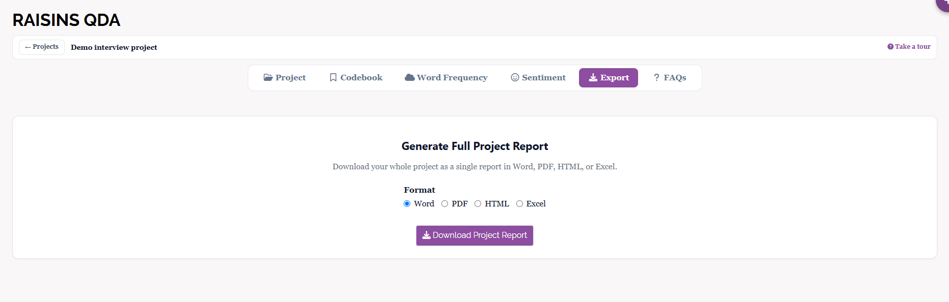
The Export tab gathers the whole project into a single report (Figure 29). Choose a Format, Word, PDF, HTML, or Excel, and click Download Project Report. The report collects the documents, the codebook, the tagged segments, and the frequency and sentiment summaries into one file, ready to attach to a thesis appendix or share with a co-author. Excel is best when you want the coded segments and counts as data for further work; Word, PDF and HTML are best for reading.
15 FAQs
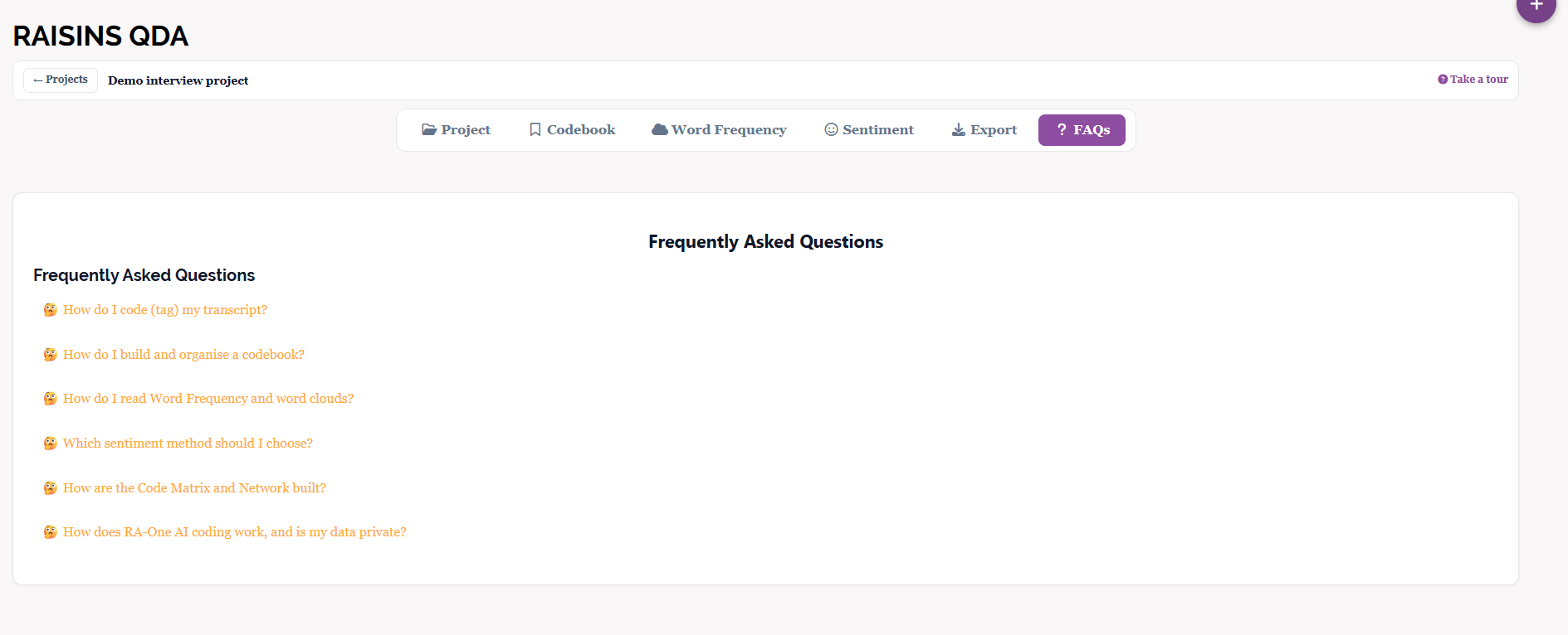
The FAQs tab answers the questions that arise most often in a first QDA project (Figure 30), among them how do I code (tag) my transcript?, how do I build and organise a codebook?, how do I read Word Frequency and word clouds?, which sentiment method should I choose?, how are the Code Matrix and Network built?, and how does RA-One AI coding work, and is my data private?. Each expands to a short explanation that restates, in one place, the guidance spread across this tutorial.
16 Wrapping up
Qualitative Data Analysis answers a different question from the numeric modules in RAISINS: not how large is an effect, but what ideas recur in this text, and how are they organised. The workflow is a single connected path, create a project, add documents, build a codebook, and tag segments (by hand or with the RA-One coder); then read the coding back through the Tagged Segments table, the codebook dashboard, word frequency, and sentiment; and finally export the whole project as one report.
Keep the coding and the summaries in dialogue with each other: the dashboards, frequencies and sentiment scores show where to look, but the meaning always lives in the passages themselves, which is why every summary in this module links back to the segments behind it. If your data are numeric rather than textual, the analysis and experiment modules are the appropriate choice instead. RA-One and the support team at [email protected] are available whenever further guidance is required.
